Wednesday, December 31, 2014

Multi-Threaded Copula producer in C#

I wanted to publish one more article for the sake of celebrating the end of the year 2014. This time I am opening one possible solution for producing multi-threaded correlated random numbers with Gaussian Copula in C#. The numerical scheme used for this procedure has already been opened well enough in this blog posting. Usually, programs presented in this blog have been having (more or less) something to do with Microsoft Excel. This time, there is only C# program. However, with all the example programs presented in this blog, the user should be able to interface this program back to Excel in many different ways, if so desired.

PRODUCER-CONSUMER


In this simple example program, Producer-Consumer Pattern has been used. CopulaQueue class is nothing more, than just a wrapper for thread-safe ConcurrentQueue data structure. More specifically, the part of the program which actually creates all correlated random numbers into CopulaQueue, is the Producer. In the program, concrete CopulaEngine implementation class takes concrete RandomGenerator implementation class and correlation matrix as its input parameters. Concrete CopulaEngine implementation class then creates correlated random numbers and uses C# Event for sending created random number matrices to CopulaQueue. Another part of the program is the Consumer. Here, I have created a simple consumer class which simply prints created random numbers to console. Consumer class also uses C# Event for Dequeueing random number matrices from CopulaQueue. Needless to say, this (Consumer) is the part of our program, where we should be utilizing all correlated random numbers created by the Producer.

On design side, this program is closely following the program presented in the blog posting referred above. Again, the beef in this design is on its flexibility to allow any new implementations for Random generator and Copula model. Moreover, our example program is using C# Framework Parallel class method Parallel.ForEach, found under System.Threading.Tasks namespace. Example program creates four producers and consumers (both into List data structure) and using multi-threading (Parallel.ForEach) when processing correlated random numbers into/from CopulaQueue.


C# PROGRAM

In order to make everything as smooth as possible for the program replication, I have been writing all required classes in the same file. Just create a new console application and copy-paste the following program into a new .cs file.

using System;
using System.Diagnostics;
using System.Linq;
using System.Collections.Generic;
using System.Threading.Tasks;
using System.Collections.Concurrent;
//
namespace MultithreadingCopula
{
    // public delegate methods needed for sending and receiving matrix data
    public delegate void MatrixSender(double[,] matrix);
    public delegate double[,] MatrixReceiver();
    // ********************************************************************
    //
    // the main program 
    class Program
    {
        static void Main(string[] args)
        {
            try
            {
                // start timer
                Stopwatch timer = new Stopwatch();
                timer.Start();
                //
                // PRODUCER PART
                // create copula implementation, correlation matrix data and list of copula engines
                CopulaQueue copulaQueue = new CopulaQueue();
                double[,] correlationMatrix = createCorrelationMatrix();
                List<CopulaEngine> engines = new List<CopulaEngine>();
                int nEngines = 4;
                int nRandomArrays = 25000;
                for (int i = 0; i < nEngines; i++)
                {
                    engines.Add(new GaussianCopula(nRandomArrays, correlationMatrix, new CSharpRandom()));
                    ((GaussianCopula)engines[i]).SendMatrix += copulaQueue.Enqueue;
                }
                // process all copula engines (producers) in parallel
                Parallel.ForEach(engines, engine => engine.Process());
                //
                // CONSUMER PART
                // create list of consumers
                List<Consumer> consumers = new List<Consumer>();
                int nConsumers = nEngines;
                for (int i = 0; i < nConsumers; i++)
                {
                    consumers.Add(new Consumer(nRandomArrays, "consumer_" + (i + 1).ToString()));
                    consumers[i].ReceiveMatrix += copulaQueue.Dequeue;
                }
                // process all consumers in parallel
                Parallel.ForEach(consumers, consumer => consumer.Process());
                //
                // stop timer, print elapsed time to console
                timer.Stop();
                Console.WriteLine("{0}  {1}", "time elapsed", timer.Elapsed.TotalSeconds.ToString());
            }
            catch (AggregateException e)
            {
                Console.WriteLine(e.Message.ToString());
            }
        }
        // hard-coded data for correlation matrix
        static double[,] createCorrelationMatrix()
        {
            double[,] correlation = new double[5, 5];
            correlation[0, 0] = 1.0; correlation[0, 1] = 0.748534249620189;
            correlation[0, 2] = 0.751; correlation[0, 3] = 0.819807151586399;
            correlation[0, 4] = 0.296516443152486; correlation[1, 0] = 0.748534249620189;
            correlation[1, 1] = 1.0; correlation[1, 2] = 0.630062355599386;
            correlation[1, 3] = 0.715491543000545; correlation[1, 4] = 0.329358787086333;
            correlation[2, 0] = 0.751; correlation[2, 1] = 0.630062355599386;
            correlation[2, 2] = 1.0; correlation[2, 3] = 0.758158276137995;
            correlation[2, 4] = 0.302715778081627; correlation[3, 0] = 0.819807151586399;
            correlation[3, 1] = 0.715491543000545; correlation[3, 2] = 0.758158276137995;
            correlation[3, 3] = 1.0; correlation[3, 4] = 0.286336231914179;
            correlation[4, 0] = 0.296516443152486; correlation[4, 1] = 0.329358787086333;
            correlation[4, 2] = 0.302715778081627; correlation[4, 3] = 0.286336231914179;
            correlation[4, 4] = 1.0;
            return correlation;
        }
    }
    // ********************************************************************
    //
    // consumer class for correlated random numbers
    public class Consumer
    {
        public event MatrixReceiver ReceiveMatrix;
        public string ID;
        private int n;
        //
        public Consumer(int n, string ID) { this.n = n; this.ID = ID; }
        public void Process()
        {
            for (int i = 0; i < n; i++)
            {
                // get correlated 1xM random matrix from CopulaQueue and print it to console
                double[,] matrix = ReceiveMatrix();
                Console.WriteLine("{0}  {1}  {2}  {3}  {4}  {5}", this.ID, Math.Round(matrix[0, 0], 4), 
                    Math.Round(matrix[0, 1], 4), Math.Round(matrix[0, 2], 4), 
                    Math.Round(matrix[0, 3], 4), Math.Round(matrix[0, 4], 4));
                //
            }
        }
    }
    // ********************************************************************
    //
    // abstract base class for all uniform random generators
    public abstract class RandomGenerator
    {
        public abstract double GetUniformRandom();
    }
    // ********************************************************************
    //
    // uniform random generator implementation by using CSharp Random class
    public class CSharpRandom : RandomGenerator
    {
        private Random generator;
        //
        public CSharpRandom()
        {
            // using unique GUID hashcode as a seed
            generator = new Random(Guid.NewGuid().GetHashCode());
        }
        public override double GetUniformRandom()
        {
            // Random.NextDouble method returns a double greater than or equal to 0.0 
            // and less than 1.0. Built-in checking procedure prevents out-of-bounds random 
            // number to be re-distributed further to CopulaEngine implementation.
            double rand = 0.0;
            while (true)
            {
                rand = generator.NextDouble();
                if (rand > 0.0) break;
            }
            return rand;
        }
    }
    // ********************************************************************
    //
    // abstract base class for all specific copula implementations
    public abstract class CopulaEngine
    {
        // Uniform random generator and correlation matrix are hosted in this abstract base class.
        // Concrete classes are providing algorithm implementation for a specific copula
        // and event mechanism for sending created correlated random numbers matrix data to CopulaQueue class.
        protected RandomGenerator generator;
        protected double[,] correlation;
        //
        public CopulaEngine(double[,] correlation, RandomGenerator generator)
        {
            this.correlation = correlation;
            this.generator = generator;
        }
        public abstract void Process();
    }
    // ********************************************************************
    //
    // concrete implementation for gaussian copula
    public class GaussianCopula : CopulaEngine
    {
        public event MatrixSender SendMatrix;
        private double[,] normalRandomMatrix;
        private double[,] choleskyMatrix;
        private double[,] correlatedNormalRandomMatrix;
        private double[,] correlatedUniformRandomMatrix;
        private int rows;
        private int cols;
        //
        public GaussianCopula(int n, double[,] correlation, RandomGenerator generator)
            : base(correlation, generator)
        {
            this.cols = base.correlation.GetUpperBound(0) + 1; // M, number of variables
            this.rows = n; // N, number of 1xM matrices
        }
        public override void Process()
        {
            // NxM matrix containing of uniformly distributed correlated random variables are calculated 
            // as a sequence of specific matrix operations
            createNormalRandomMatrix();
            createCholeskyMatrix();
            correlatedNormalRandomMatrix = MatrixTools.Transpose(MatrixTools.Multiplication(choleskyMatrix, MatrixTools.Transpose(normalRandomMatrix)));
            createCorrelatedUniformRandomMatrix();
        }
        private void createNormalRandomMatrix()
        {
            // create NxM matrix consisting of normally distributed independent random variables
            normalRandomMatrix = new double[rows, cols];
            for (int i = 0; i < rows; i++)
            {
                for (int j = 0; j < cols; j++)
                {
                    normalRandomMatrix[i, j] = StatTools.NormSInv(base.generator.GetUniformRandom());
                }
            }
        }
        private void createCholeskyMatrix()
        {
            // create lower-triangular NxM cholesky decomposition matrix
            choleskyMatrix = new double[cols, cols];
            double s = 0.0;
            //
            for (int j = 1; j <= cols; j++)
            {
                s = 0.0;
                for (int k = 1; k <= (j - 1); k++)
                {
                    s += Math.Pow(choleskyMatrix[j - 1, k - 1], 2.0);
                }
                choleskyMatrix[j - 1, j - 1] = base.correlation[j - 1, j - 1] - s;
                if (choleskyMatrix[j - 1, j - 1] <= 0.0) break;
                choleskyMatrix[j - 1, j - 1] = Math.Sqrt(choleskyMatrix[j - 1, j - 1]);
                //
                for (int i = j + 1; i <= cols; i++)
                {
                    s = 0.0;
                    for (int k = 1; k <= (j - 1); k++)
                    {
                        s += (choleskyMatrix[i - 1, k - 1] * choleskyMatrix[j - 1, k - 1]);
                    }
                    choleskyMatrix[i - 1, j - 1] = (base.correlation[i - 1, j - 1] - s) / choleskyMatrix[j - 1, j - 1];
                }
            }
        }
        private void createCorrelatedUniformRandomMatrix()
        {
            // map normally distributed numbers back to uniform plane
            // process NxM matrix row by row
            for (int i = 0; i < rows; i++)
            {
                // create a new 1xM matrix for each row and perform uniform transformation
                correlatedUniformRandomMatrix = new double[1, cols];
                for (int j = 0; j < cols; j++)
                {
                    correlatedUniformRandomMatrix[0, j] = StatTools.NormSDist(correlatedNormalRandomMatrix[i, j]);
                }
                // event : send transformed 1xM matrix to CopulaQueue
                this.SendMatrix(correlatedUniformRandomMatrix);
            }
        }
    }
    // ********************************************************************
    //
    // this is technically just a wrapper class for ConcurrentQueue data structure
    public class CopulaQueue
    {
        private ConcurrentQueue<double[,]> queue;
        public CopulaQueue()
        {
            queue = new ConcurrentQueue<double[,]>();
        }
        public void Enqueue(double[,] matrix)
        {
            // insert a matrix into data structure
            queue.Enqueue(matrix);
        }
        public double[,] Dequeue()
        {
            // remove a matrix from data structure
            double[,] matrix = null;
            bool hasValue = false;
            while (!hasValue) hasValue = queue.TryDequeue(out matrix);
            return matrix;
        }
    }
    // ********************************************************************
    //
    // collection of methods for different types of statistical calculations
    public static class StatTools
    {
        // rational approximation for the inverse of standard normal cumulative distribution. 
        // the distribution has a mean of zero and a standard deviation of one.
        // source : Peter Acklam web page home.online.no/~pjacklam/notes/invnorm/
        public static double NormSInv(double x)
        {
            const double a1 = -39.6968302866538; const double a2 = 220.946098424521;
            const double a3 = -275.928510446969; const double a4 = 138.357751867269;
            const double a5 = -30.6647980661472; const double a6 = 2.50662827745924;
            //
            const double b1 = -54.4760987982241; const double b2 = 161.585836858041;
            const double b3 = -155.698979859887; const double b4 = 66.8013118877197;
            const double b5 = -13.2806815528857;
            //
            const double c1 = -7.78489400243029E-03; const double c2 = -0.322396458041136;
            const double c3 = -2.40075827716184; const double c4 = -2.54973253934373;
            const double c5 = 4.37466414146497; const double c6 = 2.93816398269878;
            //
            const double d1 = 7.78469570904146E-03; const double d2 = 0.32246712907004;
            const double d3 = 2.445134137143; const double d4 = 3.75440866190742;
            //
            const double p_low = 0.02425; const double p_high = 1.0 - p_low;
            double q = 0.0; double r = 0.0; double c = 0.0;
            //
            if ((x > 0.0) && (x < 1.0))
            {
                if (x < p_low)
                {
                    // rational approximation for lower region
                    q = Math.Sqrt(-2.0 * Math.Log(x));
                    c = (((((c1 * q + c2) * q + c3) * q + c4) * q + c5) * q + c6) / ((((d1 * q + d2) * q + d3) * q + d4) * q + 1);
                }
                if ((x >= p_low) && (x <= p_high))
                {
                    // rational approximation for middle region
                    q = x - 0.5; r = q * q;
                    c = (((((a1 * r + a2) * r + a3) * r + a4) * r + a5) * r + a6) * q / (((((b1 * r + b2) * r + b3) * r + b4) * r + b5) * r + 1);
                }
                if (x > p_high)
                {
                    // rational approximation for upper region
                    q = Math.Sqrt(-2 * Math.Log(1 - x));
                    c = -(((((c1 * q + c2) * q + c3) * q + c4) * q + c5) * q + c6) / ((((d1 * q + d2) * q + d3) * q + d4) * q + 1);
                }
            }
            else
            {
                // throw if given x value is out of bounds (less or equal to 0.0, greater or equal to 1.0) 
                throw new Exception("input parameter out of bounds");
            }
            return c;
        }
        public static double NormSDist(double x)
        {
            // returns the standard normal cumulative distribution function. 
            // the distribution has a mean of zero and a standard deviation of one.
            double sign = 1.0;
            if (x < 0) sign = -1.0;
            return 0.5 * (1.0 + sign * errorFunction(Math.Abs(x) / Math.Sqrt(2.0)));
        }
        private static double errorFunction(double x)
        {
            // uses Hohner's method for improved efficiency.
            const double a1 = 0.254829592; const double a2 = -0.284496736;
            const double a3 = 1.421413741; const double a4 = -1.453152027;
            const double a5 = 1.061405429; const double a6 = 0.3275911;
            x = Math.Abs(x); double t = 1 / (1 + a6 * x);
            return 1 - ((((((a5 * t + a4) * t) + a3) * t + a2) * t) + a1) * t * Math.Exp(-1 * x * x);
        }
    }
    // ********************************************************************
    //
    // collection of methods for different types of matrix operations
    public static class MatrixTools
    {
        public static double[,] Transpose(double[,] matrix)
        {
            // method for transposing matrix
            double[,] result = new double[matrix.GetUpperBound(1) + 1, matrix.GetUpperBound(0) + 1];
            //
            for (int i = 0; i < matrix.GetUpperBound(0) + 1; i++)
            {
                for (int j = 0; j < matrix.GetUpperBound(1) + 1; j++)
                {
                    result[j, i] = matrix[i, j];
                }
            }
            return result;
        }
        public static double[,] Multiplication(double[,] matrix1, double[,] matrix2)
        {
            // method for matrix multiplication
            double[,] result = new double[matrix1.GetUpperBound(0) + 1, matrix2.GetUpperBound(1) + 1];
            double v = 0.0;
            //
            for (int i = 0; i < matrix1.GetUpperBound(0) + 1; i++)
            {
                for (int j = 0; j < matrix2.GetUpperBound(1) + 1; j++)
                {
                    v = 0.0;
                    for (int k = 0; k < matrix1.GetUpperBound(1) + 1; k++)
                    {
                        v += matrix1[i, k] * matrix2[k, j];
                    }
                    result[i, j] = v;
                }
            }
            return result;
        }
    }
}


TEST RUN

When running the program, I get the following console printout. The printout shows, how our four consumers used in the example program are Dequeueing correlated 1x5 random matrices from CopulaQueue in parallel.


EFFICIENCY AND CORRELATION

One million rows for 5x5 correlation matrix was processed 100 times, when testing efficiency of the producer part of the program. More specifically, four producers (CopulaEngine) are creating 1x5 matrices, consisting of five correlated uniformly distributed random numbers one by one and then sending these matrices to ConcurrentQueue wrapped in CopulaQueue class in parallel. Each of the four producers are then performing this operation 250 thousand times. Finally, the whole operation was repeated 1 hundred times and time elapsed for each repetition was saved for further analysis. The results of this experiment are reported in the table below.


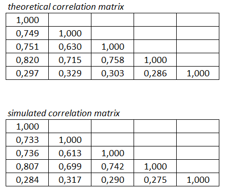
As we can see in the table, multi-threading is nicely reducing processing time, but in a non-linear fashion. Next, I printed out one batch of correlated random numbers (1000000x5 matrix) into text file and compared theoretical and simulated correlation in Excel. Results are reported in the table below. We can see, that simulated correlation is in line with theoretical correlation (enough, IMHO).


READING REFERENCES


For me personally, the following two books are standing in their own class. Ben and Joseph Albahari C# in a nutshell is presenting pretty much everything one has to know (and a lot more) about C# and especially on .NET framework. Very nice thing is also, that Albahari brothers have been kindly offering a free chapter on multi-threading from this book on their website. Daniel Duffy and Andrea Germani C# for financial markets is presenting how to apply C# in financial programs. There are a lot of extremely useful examples on multi-threaded programs, especially on using multi-threading in Monte Carlo applications and the general usage of Producer-Consumer pattern, when using multi-threading.

Again, Big thanks for reading my blog and Happy and Better New Year 2015 for everybody.

-Mike

Sunday, December 14, 2014

Write/read dynamic matrix between Excel and C# with Excel-DNA

This time I wanted to share some quick technical information about how to write or read dynamic matrix between Excel and C# program with Excel-DNA. The scheme what I am presenting here, applies to the case in which we use Excel as input/output platform for some C# program. By saying dynamic matrix, I am referring to the case, in which the dimensions of the input or output matrix are not known at compile time.

To make the long story shorter, you can use the existing program already presented in this blog posting as a base for this new example program. Just replace the content of ExcelInterface.cs file with the information given below.


C# PROGRAM

using System;
using ExcelDna.Integration;
using System.Windows.Forms;
//
namespace ExcelInterface
{
    public static class ExcelInterface
    {
        private static dynamic Excel;
        //
        public static void execute()
        {
            try
            {
                // Create Excel application and random number generator
                Excel = ExcelDnaUtil.Application;
                Random random = new Random(Guid.NewGuid().GetHashCode());
                //
                //
                //
                // CASE 1 : WRITE DYNAMIC MATRIX TO EXCEL
                int rows = (int)Excel.Range("_rows").Value2;
                int cols = (int)Excel.Range("_cols").Value2;
                double[,] matrix = new double[rows, cols];
                //
                // fill matrix with random numbers
                for (int i = 0; i < rows; i++)
                {
                    for (int j = 0; j < cols; j++)
                    {
                        matrix[i, j] = random.NextDouble();
                    }
                }
                // clear old data from output range by using Range.CurrentRegion property
                Excel.Range["_output"].CurrentRegion = "";
                //
                // resize output range to match with the dimensions of newly created random matrix
                Excel.Range["_output"].Resize[rows, cols] = matrix;
                //
                //
                //
                // CASE 2 : READ DYNAMIC MATRIX FROM EXCEL
                object[,] input = (object[,])Excel.Range["_output"].CurrentRegion.Value2;
                rows = input.GetUpperBound(0);
                cols = input.GetUpperBound(1);
                double sum = 0.0;
                //
                // sum all matrix items, calculate average and write it back to Excel
                foreach (object item in input) sum += (double)item;
                Excel.Range["_average"] = (sum / (rows * cols));
            }
            catch (Exception e)
            {
                MessageBox.Show(e.Message.ToString());
            }
        }
    }
}


In a nutshell, after creating ExcelDnaUtil.Application, we are able to use some extremely useful properties for manipulating Excel.Range object, such as CurrentRegion, Offset and Resize.

EXCEL WORKSHEET SETUPS


Dimensions for dynamic matrix output are given by the user in cells F4 and F5. Output matrix is printed to cell B8 (top left cell of output matrix). Input matrix is the same as output matrix and the C#-processed output (arithmetic average of all input matrix values) is printed into cell F6.


We have to set a couple of named Excel ranges for C# program. All the needed four named ranges are given in the screenshot below.


After implementing these range names, create a new button (Forms Controls) to this worksheet and put our C# program name into Macro box (execute). By doing this, we can get rid of the VBA code (Application.Run) completely. Any public static void method in our .NET code will be registered by Excel-DNA as a macro in Excel. Thanks for this tip to Govert Van Drimmelen (the inventor and author of Excel-DNA). After implementing all these steps, we are ready to use the program.

The purpose of this posting was to show how to handle dynamic data IO to/from Excel in C# program with Excel-DNA. For learning more things about Excel-DNA, check out its homepage. Getting more information and examples with your problems, the main source is Excel-DNA google group. Excel-DNA is an open-source project, and we (the happy users) can invest its future development by making a donation.

Thanks for reading my blog and happy waiting until Christmas.

-Mike

Friday, October 3, 2014

Calibration of short rate models in Excel with C#, Solver Foundation and Excel-DNA

This time, I wanted to present one possible solution for calibrating one-factor short interest rate model to market data. As we already know, generalized form for stochastic differential equation (SDE) for any one-factor short interest rate model is the following.


Where u and w are still undefined functions of r and t. This SDE must be solved either analytically (if such solution exists) or numerically (Monte Carlo, FDM). After solving the model, it can then be used to price different interest rate products.

The problem in these models lies in the model parameters (u, w). We could estimate those parameters from the set of market data, but in this case we (most probably) end up with a set of resulting theoretical bond prices, not matching with the corresponding market bond prices. In the case of valuing or hedging interest rate products, such prices would be then more or less useless. The second approach is to turn the whole scheme upside down. Instead of estimating parameters from the set of market data directly and then feeding those into model, we would solve a set of parameters in such a way, that our resulting theoretical bond prices will match exactly with the corresponding market bond prices. In this posting, we will solve that set of parameters numerically.

Just for a reference, full derivation of Bond Pricing Equation (BPE), plus some solutions for tractable short rate models are presented in the book written by Paul Wilmott, for example.

PROJECT OUTCOME

The end product of this small project will be C# program, which will solve numerically time-dependent theta parameters for a given short rate model (Ho-Lee as our example case) for a given set of market zero-coupon bond prices, assuming that time-dependent theta parameters are piecewise constant. C# program is using Microsoft Solver Foundation for performing the required optimization tasks. Finally, we will interface C# program into Excel workbook via VBA, with Excel-DNA.

ANALYTICAL SOLUTION FOR HO-LEE SHORT RATE MODEL


Ho-Lee model was the first no-arbitrage-type short rate model, which could be calibrated to market data. In this first section, we will go through the process of solving this SDE analytically. SDE for Ho-Lee model is the following.


Where theta is time-dependent drift coefficient (u), sigma is constant diffusion coefficient (w) and dx is the standard brownian motion. By replacing these coefficients into bond pricing equation (BPE), we get the following partial differential equation (PDE).


For this PDE, we are (very fortunately) looking for very specific solution, having the following functional form.


To solve our PDE above, we will substitute the previous solution into PDE. First, we calculate the following partial derivatives. Theta (in this case, partial derivative to time) is the following.


Delta is the following.


Gamma is the following.


After calculating partial derivatives, we substitute these into original BPE and divide all terms with V. Now we have the following PDE to be solved.


After separating all r-dependent terms and r-independent terms, we will have two ordinary differential equations (ODE) to be solved. For B coefficient, ODE is the following.


For A coefficient, ODE is the following.


After integrating ODE for B coefficient from t to T, we have the following solution.


After integrating ODE for A coefficient from t to T and substituting B coefficient into equation, we have the following solution.


We could still continue and find the exact analytical solution for time-dependent theta coefficient from this integral equation. However, for any real-life calibration purposes we have to make some assumptions concerning theta parameter. For the sake of easiness in calculations, we assume this time-dependent theta parameter to be piecewise constant. With this assumption, we get the following solution for A coefficient.


After integrating the last existing integral term, we have the following solution for A coefficient.


Finally, we have the following functional form for a zero-coupon bond price according to Ho-Lee, which can be used for calibration purposes.


From this equation, we could also solve for the unknown theta parameter analytically, without any numerical methods involved.


CALIBRATION

The pricing process with models usually starts with some already known parameters, which are then feeded into some model to calculate the results. For example, in the case of Ho-Lee model, we would know the values for spot rate, time-dependent theta, constant sigma and bond maturity. Then, by calculating coefficients A and B we would calculate zero-coupon bond price and the corresponding yield.

Concerning short rate models, these parameters are usually not known in advance and have to be estimated or calibrated. In the calibration process, we are performing the whole pricing process backwards. First, we know the market yield for a zero-coupon bond. From this yield we calculate the corresponding bond price. Assuming that we know (or have been estimating) the values for spot rate, maturity and constant sigma parameter, we can then solve for coefficient A and B. Finally, we can calculate the value for time-dependent theta parameter.

Consider the case, in which we have Libor zero curve as our input market data, consisting of N zero-coupon bond yields. From this curve, we calculate the corresponding N zero-coupon bond prices. Consider also, that we have statistically estimated the value for constant sigma (standard deviation of a short rate) and we know spot rate and N maturities. After this, we set N initial values for our piecewise constant theta parameters. By using these theta parameters, we then calculate N pairs of A and B coefficients. Finally, N theoretical bond prices and N theoretical yields can be calculated by using N pairs of A and B coefficients. In the final stage, we just adjust our initial values for our N piecewise constant theta parameters, until theoretical yields and corresponding market yields are equal for all N bonds. More specifically, we minimize the sum of absolute squared errors between theoretical yields and corresponding market yields. This part is just unconstrained minimization problem. As a result of this minimization we will solve N theta parameters, for which theoretical bond prices are matching exactly with market bond prices. In other words, we are calibrating our model to market data.

As already noted above, we are dealing with the model having analytical solution (affine or tractable models). In this case, there is actually no need for any numerical method when calibrating model parameters to market. However, for the sake of curiosity and craftmanship, we will perform this calibration process numerically.


PREPARATORY TASKS

Next, we have to get the tools for performing optimization needed in the calibration process. As a proud holder of the NAG licence, I would use these numerical libraries for the task. However, in this project we will use Microsoft Solver Foundation, since it is freely available without any costs involved. Next, download Solver Foundation solver (32-bit). If this package is completely alien for you, there are excellent hands-on tutorials available, written by Mathias Brandewinder in here and in here. Replicating and studying these examples will get you started with Solver Foundation.

Also, download and unzip Excel-DNA Version 0.30 zip file to be ready when needed. This is the version I have been using so far, but I assume you can also use newer version 0.32. Concerning the tools needed, we are now ready to move on to create the actual C# program.


PROGRAM DESIGN

Design for C# program has been presented in the following UML chart. In order to understand better what is happening between the objects, some comments are given inside the blue boxes. The main point in this design is its flexibility to handle new one-factor models. This example has been specifically made using Ho-Lee model. However, user is able to create new implementations for CIR or Vasicek model, if needed.


C# PROGRAM

Create a new C# Class project "SolverApp_25092014". Target framework is .NET Framework 4. Remember also to create a new reference into SolverFoundation dll file (Project - Add reference - Browse - \Microsoft.Solver.Foundation.dll). My dll file is found within the following folder: C:\Program Files (x86)\Reference Assemblies\Microsoft\Framework\.NETFramework\v4.0\Microsoft.Solver.Foundation.dll. The workhorse classes for this program are presented below. Create new class files and copyPaste the following codes into separate classes.

using System;
using System.Collections.Generic;
using System.Linq;
using System.Text;
using Microsoft.SolverFoundation.Services;

namespace SolverApp_25092014
{
    public interface IOneFactorModel
    {
        Term price(Term parameter, Term t);
    }
}


using System;
using System.Collections.Generic;
using System.Linq;
using System.Text;
using Microsoft.SolverFoundation.Services;

namespace SolverApp_25092014
{
    public abstract class OneFactorModel : IOneFactorModel
    {
        public abstract Term price(Term parameter, Term t);
    }
}


using System;
using System.Collections.Generic;
using System.Linq;
using System.Text;
using Microsoft.SolverFoundation.Services;

namespace SolverApp_25092014
{
    public class HoLee : OneFactorModel
    {
        private Term spot;
        private Term stdev;
        //
        public HoLee(double spot, double stdev)
        {
            this.stdev = stdev; this.spot = spot;
        }
        public override Term price(Term parameter, Term t)
        {
            // create term object for Ho-Lee bond price for a given eta and t
            Term B = t;
            Term c1 = Model.Quotient(1, 2);
            Term c2 = Model.Quotient(1, 6);
            Term A = -(parameter * (c1 * Model.Power(t, 2))) + c2 * Model.Power(stdev, 2) * Model.Power(t, 3);
            return Model.Exp(A - spot * B);
        }
    }
}


using System;
using System.Collections.Generic;
using System.Linq;
using System.Text;
using Microsoft.SolverFoundation.Services;

namespace SolverApp_25092014
{
    public class OneFactorCalibrator
    {
        private OneFactorModel model;
        private Dictionary<double, double> curve;
        //
        public OneFactorCalibrator(OneFactorModel model, Dictionary<double, double> curve)
        {
            this.model = model; this.curve = curve;
        }
        public List<double> calibrate()
        {
            // create a new solver model
            SolverContext solver = new SolverContext();
            solver.ClearModel();
            Model solverModel = solver.CreateModel();
            //
            // create decision variables, a set of parameters to be calibrated
            var decisions = curve.Select(it => new Decision(Domain.Real, "parameter_" + it.Key.ToString()));
            solverModel.AddDecisions(decisions.ToArray());
            //
            // create objective function as sum of differences between market and theoretical yields
            SumTermBuilder terms = new SumTermBuilder(curve.Count);
            int i = 0;
            foreach (KeyValuePair<double, double> kvp in curve)
            {
                // define required term objects
                Term eta = solverModel.Decisions.ElementAt(i++);
                Term t = kvp.Key;
                //
                // calculate bond prices and yields
                Term theoreticalPrice = model.price(eta, t);
                Term theoreticalYield = Model.Power(Model.Quotient(1, theoreticalPrice), Model.Quotient(1, t)) - 1;
                Term marketPrice = kvp.Value;
                Term marketYield = Model.Power(Model.Quotient(1, marketPrice), Model.Quotient(1, t)) - 1;
                Term yieldDifference = Model.Power(marketYield - theoreticalYield, 2);
                //
                // add constructed term into sumbuilder (objective function)
                terms.Add(yieldDifference);
            }
            //
            // define optimization goal, solve the model and pack results into list
            solverModel.AddGoal("solverGoal", GoalKind.Minimize, Model.Abs(terms.ToTerm()));
            Solution result = solver.Solve();
            return solverModel.Decisions.Select(it => it.ToDouble()).ToList();
        }
    }
}

At this point, we should be able to build this class project without any errors or warnings. The only thing that might create a bit of confusion here, is the logic of using Solver Foundation and especially its Term object. If you feel uncomfortable using solver objects, you may spend some quality time and go through examples by Mathias Brandewinder mentioned earlier. Also, going through the stuff presented in Microsoft.Solverfoundation.Services Namespace relieves the painful climbing on this new learning curve. There are also some documentation pdf files included in the downloaded package from Microsoft. Anyway, the basic functionality for calibration process has now been set. Next, we have to interface our C# program and Excel.


Excel-DNA

Concerning the usage and creating interface between Excel and C#, we are following instructions presented in this blog posting.

Add reference to Excel-DNA library (Project - Add reference - Browse - \\ExcelDna.Integration.dll) and click OK. This dll file is inside the distribution folder what we just downloaded from Excel-DNA  website. From the properties of this reference, set Copy Local to be False.

Add new file as text file to project (Project - Add new item - Text file) and name it to be SolverApp_25092014.dna. CopyPaste the following xml code into this file.

<DnaLibrary Name="SolverApp_25092014" RuntimeVersion="v4.0">
  <ExternalLibrary Path="SolverApp_25092014.dll" />
</DnaLibrary>

From the properties of this dna file, set Copy to Output Directory to be Copy if newer.

Next, from the downloaded Excel-DNA folder (Distribution), copy ExcelDna.xll file into your project folder (\\Projects\SolverApp_25092014\SolverApp_25092014) and rename it to be SolverApp_25092014.xll. Then, add this xll file into your current project (Project - Add existing item). At this point, it might be that you do not see anything else, except cs files on this window. From drop down box on the bottom right corner of this window, select All files and you should see ExcelInterface.xll file what we just pasted into this ExcelInterface folder. Select this file and press Add. Finally, from the properties of this xll file, set Copy to Output Directory to be Copy if newer.

Build the solution. Again, everything should have gone well without any errors or warnings. At this point, my \\SolverApp_25092014\bin\Release folder looks like the following.


Next, we start to build interface between C# program and Excel workbook, via VBA


EXCEL USER INTERFACE AND C#-VBA INTEGRATION

Add new class into project and name it to be "SolverApp_25092014". Remember also, that we might need to use Message Box for error reporting coming from catch block. Hence, we need to create reference to System.Windows.Forms library (Project - Add reference - .NET - System.Windows.Forms). CopyPaste the following code into this new class file. After this, build solution again and save it. We should be able to rebuild this class project again without any errors or warnings.

using System;
using System.Collections.Generic;
using System.Linq;
using System.Text;
using System.Windows.Forms;
using ExcelDna.Integration;

namespace SolverApp_25092014
{
    public static class SolverApp_25092014
    {
        public static void calibrate()
        {
            try
            {
                // create Excel application object
                dynamic Excel = ExcelDnaUtil.Application;
                //
                // read scalar parameters from named ranges
                double r = (double)Excel.Range["_r"].Value2;
                double stdev = (double)Excel.Range["_stdev"].Value2;
                //
                // read curve from named range
                dynamic Matrix = Excel.Range["_curve"].Value2;
                int rows = Matrix.GetUpperBound(0);
                //
                // export curve data into dictionary
                Dictionary<double, double> curve = new Dictionary<double, double>();
                for (int i = 0; i < rows; i++)
                {
                    double key = (double)Matrix.GetValue(i + 1, 1);
                    double value = (double)Matrix.GetValue(i + 1, 2);
                    curve.Add(key, value);
                }
                //
                // create model and calibrator instances
                OneFactorModel model = new HoLee(r, stdev);
                OneFactorCalibrator calibrator = new OneFactorCalibrator(model, curve);
                List<double> theta = calibrator.calibrate();
                //
                // export theta parameters into 2-dimensional array
                double[,] result = new double[rows, 1];
                for (int i = 0; i < theta.Count; i++) result[i, 0] = theta[i];
                //
                // print array into named range
                Excel.Range["_theta"] = result;
            }
            catch (Exception e)
            {
                MessageBox.Show(e.Message.ToString());
            }
        }
    }
}


We are almost there. Next, we will create Excel worksheet interface and VBA "trigger program" for C# program. The action starts as the user is pressing commandbutton, which then calls a simple VBA program, which then triggers the actual C# workhorse program. Create the following data view into a new Excel worksheet. Also, insert command button into worksheet.


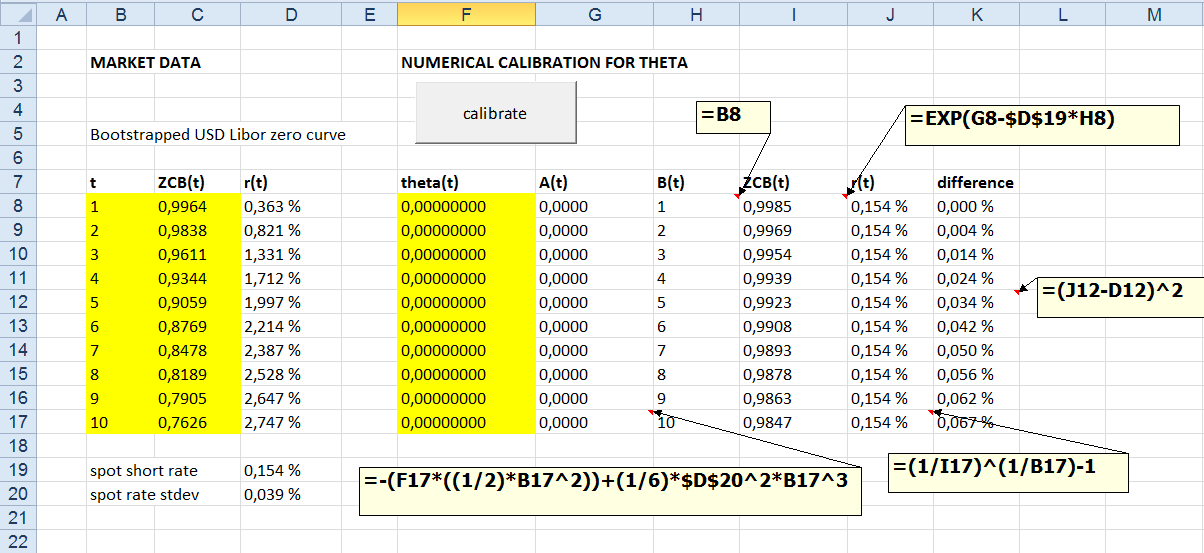
A few words concerning this worksheet. Zero-coupon bond curve maturities and prices are given in the columns B and C (yellow). Corresponding yields are calculated in the column D. Vector of time-dependent piecewise constant thetas will be calibrated and printed into column F (yellow). Columns from G to K are using analytical solution for Ho-Lee model to calculate theoretical zero-coupon bond prices and yields. Squared differences between market yields and calculated theoretical yields are given in the column K.

Input (output) data for (from) C# program are going to be read (written) directly from (to) Excel named ranges. Create the following named Excel ranges.


Finally, insert a new standard VBA module and create simple program calling the actual C# program (Sub tester). Also, create event-handling program for commandbutton click, which then calls the procedure shown below.


Concerning the program and its interfacing with Excel, all those small pieces have finally been assembled together. Now, it is time to do the actual calibration test run.


TEST RUN AND MODEL VALIDATION

In this section we will perform test run and check, whether our calibration model is working properly. In another words, are we able to replicate the market with our model. After pressing "calibrate" button, my Excel shows the following calibration results for theta parameters shown in column F.


Analytical results are already calculated in the worksheet (columns G to J). For example, time-dependent theta parameter for 4 years is 0.00771677. With this theta value embedded in A coefficient will produce zero-coupon bond price, equal to corresponding market price.

How about using SDE directly with these calibrated time-dependent thetas? Let us use Monte Carlo to price 4-year zero-coupon bond by using SDE directly. For the sake of simplicity, we perform this exercise in Excel. Simulation scheme is presented in the screenshot below.


In this Excel worksheet presented above, 4-year period has been divided into 800 time steps, which gives us the size for one time step to be 0.005 years. Total of 16 378 paths was simulated by using Ho-Lee SDE with calibrated time-dependent piecewise constant theta parameter. All simulated zero-coupon bond prices have been calculated in the row 805. By taking the average for all these 16 378 simulated zero-coupon bond prices, gives us the value of 0.9343. Needless to say this value is  random variable, which changes every time we press that F9 button. Our corresponding market price for 4-year zero-coupon bond is 0.9344, so we are not far away from that value. We can make the conclusion, that our calibration is working as expected.

Thanks for reading this blog.
-Mike

Saturday, August 16, 2014

Bootstrapping OIS-adjusted Libor curve in VBA

OIS discounting has been hot topic for the last few years, since most of the collateralized OTC swaps are valued by this methodology. In this blog post, I will present simple example algorithm for bootstrapping OIS-adjusted Libor curve from market data (OIS zero-coupon curve, Libor par swap curve). This bootstrapped curve can then be used to generate floating leg cash flows, when valuing collateralized interest rate swap with all cash flows and collateral in the same currency. Final product will be just one simple VBA worksheet function to be used in Excel.

VALUATION 101

In essence
  • Instead of using Libor zero-coupon curve for cash flow discounting, all swap cash flows are present valued with discount factors calculated by using OIS zero-coupon curve. 
  • The use of OIS zero-coupon curve for discounting collateralized swap cash flows is justified, because posted collateral earns overnight rate and collateral value is mark-to-market value of a swap. In order to equate these two cash flows (collateral value, mark-to-market value of a swap), discount factor for both cash flows has to be calculated by using OIS curve.
  • Cash flows for swap fixed leg are still constructed by using ordinary Libor par swap rates. 
  • Another impact of OIS valuation hits into construction of floating leg coupon rates, which are technically forward rates.
  • In the "old world", we bootstrapped Libor zero-coupon curve, from which we calculated discount factors and forward rates (for constructing floating leg coupons) at the same time. Only one curve was needed to accomplish this procedure. 
  • Because all swap cash flows are now discounted with OIS zero-coupon curve and ordinary Libor par swap rates are still used for constructing swap fixed leg cash flows, forward rates have to be "adjusted" slightly, in order to equate present value of all swap cash flows to be zero.
  • Technically, we end up with a system of linear equations, in which we equate OIS-discounted floating cash flows with OIS-discounted fixed cash flows and solve for the unknown forward rates.
Material, which has helped me to understand this subject a bit better is the following: technical notes written by Justin Clarke, teaching material by Donald J. Smith and Barclays research paper by Amrut Nashikkar. These papers have worked numerical examples, as well as theoretical issues covered thoroughly.

VBA FUNCTION


Option Explicit
'
Public Function OIS_bootstrapping(ByRef curves As Range) As Variant
    '
    ' import source data from Excel range into matrix
    Dim source As Variant: source = curves.Value2
    '
    ' create all the needed matrices and define dimensions
    Dim nSwaps As Integer: nSwaps = UBound(source, 1)
    Dim fixed As Variant: ReDim fixed(1 To nSwaps, 1 To 1)
    Dim float As Variant: ReDim float(1 To nSwaps, 1 To nSwaps)
    Dim forward As Variant: ReDim forward(1 To nSwaps, 1 To 1)
    '
    ' counters and other temp variables
    Dim i As Integer, j As Integer, k As Integer, nCashFlows As Integer
    Dim OIS_DF As Double, OIS_Rate As Double, t As Double
    '
    ' loop for cash flows processing
    nCashFlows = nSwaps: k = 0
    For i = 1 To nSwaps
        '
        ' create OIS discount factor
        OIS_Rate = source(i, 2): t = source(i, 1)
        If (t <= 1) Then OIS_DF = 1 / (1 + (OIS_Rate * t))
        If (t > 1) Then OIS_DF = 1 / (1 + OIS_Rate) ^ t
        '
        ' create sum of fixed leg pv's for each individual swap and create all
        ' cash flows (excluding coupon rate) for floating legs for each individual swap
        For j = 1 To nSwaps
            If (j <= nCashFlows) Then
                fixed(j + k, 1) = fixed(j + k, 1) + 100 * source(j + k, 3) * OIS_DF
                float(i, j + k) = 100 * OIS_DF
            Else
                ' replace empty array value with zero value
                float(i, nSwaps - j + 1) = 0#
            End If
        Next j
        '
        k = k + 1: nCashFlows = nCashFlows - 1
    Next i
    '
    ' solve for implied forward rates, which are going to be used to generate coupons
    ' for floating legs. matrix operation: [A * x = b] ---> [x = Inverse(A) * b]
    ' where A = float (N x N), x = forward rates (N x 1), b = sum of swap fixed leg pv's (N x 1)
    forward = WorksheetFunction.MMult(WorksheetFunction.MInverse(WorksheetFunction.transpose(float)), fixed)
    OIS_bootstrapping = forward
End Function
'


EXAMPLE CALCULATION


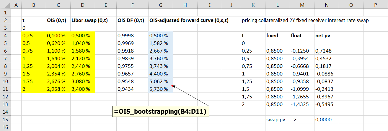
The following Excel screenshot presents bootstrapped OIS-adjusted forward curve (column G) and OIS valuation for collateralized 2Y interest rate swap. For the sake of simplicity, this example assumes that the payments for the both fixed and floating legs takes place quarterly. Swap fixed cash flows has been constructed by using Libor par swap rates. Floating leg cash flows has been constructed by using bootstrapped OIS-adjusted forward curve. Finally, all cash flows are discounted by using OIS discount factors (column F). The present value of all swap cash flows is zero. Worksheet function input range has been marked with yellow color and function output range has been marked with blue color.


Presented forward curve construction scheme applies to a specific case, in which collateralized interest rate swap has the both cash flow legs and collateral in the same currency. Moreover, it is assumed that the payment frequency is the same for the both swap legs. Successful replication of the forward curve bootstrapping result was achieved, when testing VBA worksheet function with the cases presented in above-mentioned papers by Smith and Clarke.

Thanks for reading.

-Mike