AlgLib : Ho-Lee Calibration Using Levenberg-Marquardt algorithm in VBA

Some time ago, I published one possible C# implementation for Ho-Lee one-factor model calibration scheme using AlgLib numerical libraries. This time I will present an implementation for the same scheme in VBA. General information concerning Levenberg-Marquardt algorithm implementation in AlgLib has been presented in here. Libraries for VBA (collection of BAS module files, which are going to be included into VBA project) can be downloaded from here.

A few words about this implementation. AlgLibLMASolver class uses AlgLib library functions (functions from 21 different modules) for processing (creating optimization model, setting conditions, processing iterations). One data member within this class is having a type of IModel. This data member is actually a reference to an interface, which provides a set of functions for all required calculations (objective function value, values for function terms, partial derivative values for function terms). Since all possible implementations for any interface method must honor signatures exactly, there is a problem with VBA since it does not have a real constructor mechanism. I have chewed this issue in here. It might help to explain the reason, why I have been distributing input parameters for interface implementation by using Dictionary object. Finally, HoLeeZeroCouponCalibration class is implementing IModel interface (a set of functions for all required calculations). In essence, algorithms (AlgLib-related processing) and data (values calculated specifically by using Ho-Lee model) have been completely separated. Needless to say, this type of scheme is flexible for new implementations.

Create a new VBA project and copy-paste the following classes and modules into this project. Also, import all required 21 AlgLib BAS files into this project.

' CLASS : AlgLibLMASolver
Option Explicit
'
' The following 21 AlgLib modules are required for succesfull compilation of this project :
' ablas, ablasf, ap, bdsvd, blas, creflections, densesolver, hblas, linmin, matinv,
' minlbfgs, minlm, ortfac, rcond, reflections, rotations, safesolve, sblas, svd, trfac, xblas
'
Private state As MinLMState
Private report As MinLMReport
Private n As Long
Private m As Long
Private x() As Double
Private model As IModel
Private epsF As Double
Private epsG As Double
Private epsX As Double
Private iterations As Long
'
Public Function initialize( _
    ByVal numberOfVariables As Long, _
    ByVal numberOfEquations As Long, _
    ByRef changingVariables() As Double, _
    ByRef callbackModel As IModel, _
    ByVal epsilonF As Double, _
    ByVal epsilonG As Double, _
    ByVal epsilonX As Double, _
    ByVal maximumIterations As Long)
    '
    n = numberOfVariables
    m = numberOfEquations
    x = changingVariables
    Set model = callbackModel
    epsF = epsilonF
    epsG = epsilonG
    epsX = epsilonX
    iterations = maximumIterations
End Function
'
Public Sub Solve()
    '
    ' create solver scheme using functions and analytical partial derivatives
    Call MinLMCreateFJ(n, m, x, state)
    ' set stopping conditions
    Call MinLMSetCond(state, epsG, epsF, epsX, iterations)
    '
    ' process iterations
    Do While MinLMIteration(state)
        '
        ' calculate value for objective function
        If (state.NeedF) Then
            '
            model.callBackObjectiveFunction state
        End If
        '
        ' calculate values for functions and partial derivatives
        If (state.NeedFiJ) Then
            '
            model.callBackFunction state
            model.callBackJacobian state
        End If
    Loop
    '
    ' process results
    Call MinLMResults(state, x, report)
End Sub
'
' public accessor to (MinLMState) state
Public Property Get GetState() As MinLMState
    GetState = state
End Property
'
' public accessor to (MinLMReport) report
Public Property Get GetReport() As MinLMReport
    GetReport = report
End Property
'
' public accessor to hard-coded report
Public Property Get GetPrettyPrintReport() As String
    '
    Dim message As String
    message = "*** AlgLibLMASolver execution report " + VBA.CStr(VBA.Now) + " ***" + VBA.vbNewLine
    message = message + "TerminationType : " + VBA.CStr(report.TerminationType) + VBA.vbNewLine
    message = message + "Iterations : " + VBA.CStr(report.IterationsCount) + VBA.vbNewLine
    message = message + "Objective function : " + VBA.CStr(state.f) + VBA.vbNewLine
    message = message + VBA.vbNewLine
    '
    Dim i As Integer
    For i = 0 To (state.n - 1)
        message = message + "x(" + VBA.CStr(i) + ") = " + VBA.CStr(state.x(i)) + VBA.vbNewLine
    Next i
    '
    GetPrettyPrintReport = message
End Property
'
'
'
'
'
' CLASS : IModel
Option Explicit
' set of functions for IModel interface
Public Function initialize(ByRef parameters As Scripting.Dictionary)
    ' assign required member data wrapped into dictionary
End Function
'
Public Function callBackObjectiveFunction(ByRef state As MinLMState)
    ' calculate objective function value
End Function
'
Public Function callBackFunction(ByRef state As MinLMState)
    ' calculate values for (non-squared) function terms
End Function
'
Public Function callBackJacobian(ByRef state As MinLMState)
    ' calculate partial derivative values for (non-squared) function terms
End Function
'
'
'
'
'
' CLASS : HoLeeZeroCouponCalibration
Option Explicit
'
Implements IModel
'
Private s As Double
Private r As Double
Private t() As Double
Private z() As Double
'
Private Function IModel_initialize(ByRef parameters As Scripting.IDictionary)
    '
    s = parameters(HOLEE_PARAMETERS.sigma)
    r = parameters(HOLEE_PARAMETERS.shortRate)
    t = parameters(HOLEE_PARAMETERS.maturity)
    z = parameters(HOLEE_PARAMETERS.zeroCouponBond)
End Function
'
Private Function IModel_callBackObjectiveFunction(ByRef state As MinLMState)
    '
    ' calculate value for aggregate objective function
    Dim i As Integer
    Dim hoLeeZero As Double
    Dim f As Double: f = 0
    '
    ' loop through number of equations
    For i = 0 To (state.m - 1)
        '
        hoLeeZero = VBA.Exp(-(1 / 2) * state.x(i) * (t(i) ^ 2) + (1 / 6) * (s ^ 2) * (t(i) ^ 3) - r * t(i))
        f = f + (z(i) - hoLeeZero) ^ 2
    Next i
    state.f = f
End Function
'
Private Function IModel_callBackFunction(ByRef state As MinLMState)
    '
    ' calculate values for (non-squared) function terms
    Dim i As Integer
    Dim hoLeeZero As Double
    '
    ' loop through number of equations
    For i = 0 To (state.m - 1)
        '
        hoLeeZero = VBA.Exp(-(1 / 2) * state.x(i) * (t(i) ^ 2) + (1 / 6) * (s ^ 2) * (t(i) ^ 3) - r * t(i))
        state.FI(i) = (z(i) - hoLeeZero)
    Next i
End Function
'
Private Function IModel_callBackJacobian(ByRef state As MinLMState)
    '
    ' calculate partial derivative values for (non-squared) function terms
    Dim i As Integer, J As Integer
    Dim hoLeeZero As Double
    '
    ' 1. individual (non-squared) function terms
    ' loop through number of equations
    For i = 0 To (state.m - 1)
        '
        hoLeeZero = VBA.Exp(-(1 / 2) * state.x(i) * (t(i) ^ 2) + (1 / 6) * (s ^ 2) * (t(i) ^ 3) - r * t(i))
        state.FI(i) = (z(i) - hoLeeZero)
    Next i
    '
    ' 2. partial derivatives for all (non-squared) function terms
    ' loop through number of equations
    For i = 0 To (state.m - 1)
        '
    ' loop through number of variables
        For J = 0 To (state.n - 1)
            '
            Dim derivative As Double: derivative = 0
            ' partial derivative is non-zero only for diagonal cases
            If (i = J) Then
                derivative = (1 / 2) * VBA.Exp(1) * t(J) ^ 2
                state.J(i, J) = derivative
            End If
        Next J
    Next i
End Function
'
'
'
'
'
' MODULE : DataStructures
Option Explicit
'
Public Enum HOLEE_PARAMETERS
    sigma = 1
    shortRate = 2
    maturity = 3
    zeroCouponBond = 4
End Enum
'
'
'
'
'
' TESTER MODULE
Option Explicit
'
' Ho-Lee model calibration example
Public Sub AlglibTester()
    '
    ' MODEL part
    ' construct all required inputs and model to be calibrated
    Dim sigma As Double: sigma = 0.00039
    Dim shortRate As Double: shortRate = 0.00154
    '
    Dim maturity(0 To 9) As Double
    maturity(0) = 1: maturity(1) = 2: maturity(2) = 3: maturity(3) = 4: maturity(4) = 5:
    maturity(5) = 6: maturity(6) = 7: maturity(7) = 8: maturity(8) = 9: maturity(9) = 10
    '
    Dim zero(0 To 9) As Double
    zero(0) = 0.9964: zero(1) = 0.9838: zero(2) = 0.9611: zero(3) = 0.9344: zero(4) = 0.9059:
    zero(5) = 0.8769: zero(6) = 0.8478: zero(7) = 0.8189: zero(8) = 0.7905: zero(9) = 0.7626
    '
    ' assign parameters into dictionary wrapper
    Dim parameters As New Scripting.Dictionary
    parameters.Add HOLEE_PARAMETERS.sigma, sigma
    parameters.Add HOLEE_PARAMETERS.shortRate, shortRate
    parameters.Add HOLEE_PARAMETERS.maturity, maturity
    parameters.Add HOLEE_PARAMETERS.zeroCouponBond, zero
    '
    ' create and initialize calibration model
    Dim model As IModel: Set model = New HoLeeZeroCouponCalibration
    model.initialize parameters
    '
    ' SOLVER part
    Dim Theta(0 To 9) As Double ' assign initial guesses
    Theta(0) = 0.001: Theta(1) = 0.001: Theta(2) = 0.001: Theta(3) = 0.001: Theta(4) = 0.001:
    Theta(5) = 0.001: Theta(6) = 0.001: Theta(7) = 0.001: Theta(8) = 0.001: Theta(9) = 0.001
    '
    Dim numberOfVariables As Long: numberOfVariables = 10
    Dim numberOfEquations As Long: numberOfEquations = 10
    Dim epsilonF As Double: epsilonF = 0.000000000001
    Dim epsilonG As Double: epsilonG = 0.000000000001
    Dim epsilonX As Double: epsilonX = 0.000000000001
    Dim maximumIterations As Long: maximumIterations = 25000
    '
    ' create and initialize solver model
    Dim solver As New AlgLibLMASolver
    solver.initialize _
        numberOfVariables, _
        numberOfEquations, _
        Theta, _
        model, _
        epsilonF, _
        epsilonG, _
        epsilonX, _
        maximumIterations
    '
    ' solve calibration model
    solver.Solve
    '
    ' print hard-coded report containing values for
    ' objective function, variables and other information
    Debug.Print solver.GetPrettyPrintReport
End Sub
'

The results from this calibration model have been verified against the previous results.

Importing several files into project may involve considerable amount of cruel and unusual repetitive labour. For this specific reason, I have also been woodshedding a separate module (employing VBIDE object), which might give some relief when babysitting those AlgLib modules.

' The following dll libraries need to be referenced :
' Microsoft Visual Basic for Applications Extensibility 5.X, Microsoft Scripting Runtime
Option Explicit
Option Base 0
'
' address to a list, which contains all BAS files which will be included into project
Const listFolderPathName As String = "C:\AlgLib\vba\AlgLibLMAModules.txt"
' address to a folder, which contains all AlgLib BAS files
Const moduleFolderPathName  As String = "C:\AlgLib\vba\alglib-2.6.0.vb6\vb6\src\"
' select TRUE, if Require Variable Declaration in editor is tagged
Const removeOptionExplicitDirective As Boolean = True
'
Public Sub ImportModules()
    '
    ' create a list of modules to be imported into this project
    Dim list() As String: list = createProjectModuleList
    ' import modules into active project
    import list
End Sub
'
Public Sub ExportModules()
    '
    ' create a list of modules to be exported from this project
    Dim list() As String: list = createProjectModuleList
    ' export modules from active project into a defined folder
    export list
End Sub
'
Public Sub RemoveModules()
    '
    ' create a list of modules to be removed from this project
    Dim list() As String: list = createProjectModuleList
    ' delete modules from active project
    remove list
End Sub
'
Private Function import(ByRef list() As String)
    '
    Dim editor As VBIDE.VBProject
    Set editor = ActiveWorkbook.VBProject
    Dim fileSystem As Scripting.FileSystemObject: Set fileSystem = New Scripting.FileSystemObject
    '
    ' loop through all files in a specific source folder for modules
    Dim filesInGivenList As Integer: filesInGivenList = UBound(list) + 1
    If (filesInGivenList = 0) Then Exit Function
    '
    Dim module As VBIDE.VBComponent
    Dim file As Scripting.file
    For Each file In fileSystem.GetFolder(moduleFolderPathName).Files
        '
        ' if there is a given list of specific files to be included
        ' select only the files in that list to be imported into project
        If Not (moduleIsIncluded(file.Name, list)) Then GoTo skipPoint
        '
        Set module = editor.VBComponents.Add(vbext_ct_StdModule)
        If (removeOptionExplicitDirective) Then module.CodeModule.DeleteLines 1
        module.Name = VBA.Split(file.Name, ".")(0)
        module.CodeModule.AddFromFile file.Path
skipPoint:
    Next
End Function
'
Private Function export(ByRef list() As String)
    '
    Dim filesInGivenList As Integer: filesInGivenList = UBound(list) + 1
    If (filesInGivenList = 0) Then Exit Function
    '
    Dim editor As VBIDE.VBProject
    Set editor = ActiveWorkbook.VBProject
    Dim module As VBIDE.VBComponent
    '
    ' loop through all modules
    For Each module In editor.VBComponents
        '
        ' export module only if it is included in the list
        If (moduleIsIncluded(module.Name + ".bas", list)) Then
            module.export moduleFolderPathName + module.Name + ".bas"
        End If
    Next
End Function
'
Private Function remove(ByRef list() As String)
    '
    Dim filesInGivenList As Integer: filesInGivenList = UBound(list) + 1
    If (filesInGivenList = 0) Then Exit Function
    '
    Dim editor As VBIDE.VBProject
    Set editor = ActiveWorkbook.VBProject
    Dim module As VBIDE.VBComponent
    '
    ' loop through all modules
    For Each module In editor.VBComponents
        '
        ' remove module only if it is included in the list
        If (moduleIsIncluded(module.Name + ".bas", list)) Then
            module.Collection.remove module
        End If
    Next
End Function
'
Private Function moduleIsIncluded(ByVal FileName As String, ByRef list() As String) As Boolean
    '
    ' check if a given file name is in the list
    Dim isIncluded As Boolean: isIncluded = False
    Dim i As Integer
    For i = 0 To UBound(list)
        If (FileName = list(i)) Then
            isIncluded = True
            Exit For
        End If
    Next i
    moduleIsIncluded = isIncluded
End Function
'
Private Function createProjectModuleList() As String()
    '
    ' create a list of file names from text file
    Dim fileSystem As Scripting.FileSystemObject: Set fileSystem = New Scripting.FileSystemObject
    Dim fileReader As Scripting.TextStream: Set fileReader = fileSystem.OpenTextFile(listFolderPathName, ForReading)
    Dim fileStreams As String: fileStreams = fileReader.ReadAll
    Dim streams As Variant: streams = VBA.Split(fileStreams, VBA.vbNewLine)
    Dim list() As String: ReDim list(0 To UBound(streams))
    Dim i As Integer
    For i = 0 To UBound(streams)
        list(i) = VBA.Trim(streams(i))
    Next i
    createProjectModuleList = list
End Function
'

Finally, thanks for reading this blog.
-Mike

Alglib : Ho-Lee calibration in C#

A couple of years ago I published post on Ho-Lee short interest rate model calibration using Microsoft Solver Foundation (MSF). Solver is still available (somewhere) but not supported or developed any further, since Microsoft terminated that part of their product development (if I have understood the story correctly). As a personal note I have to say, that MSF was actually not the easiest package to use, from programming point of view.

Life goes on and very fortunately there are a lot of other alternatives available. This time I wanted to present Alglib, which is offering quite impressive package of numerical stuff already in their non-commercial (free of charge) edition. In optimization category, there is Levenberg-Marquardt algorithm (LMA) implementation available, which can be used for multivariate optimization tasks. Within this post, I am re-publishing short interest rate model calibration scheme, but only using Alglib LMA for performing the actual optimization routine.

In the case that Alglib is completely new package, it is recommended to check out some library documentation first, since it contains a lot of simple "Copy-Paste-Run"-type of examples, which will help to understand how the flow of information is processed. As a personal note I have to say, that time and effort needed to "getting it up and running" is extremely low. Just find Alglib download page, download proper C# version, create a new C# project and add reference to DLL file (alglibnet2.dll) included in download folder.

The outcome

Market prices of zero-coupon bonds, volatility (assumed to be estimated constant) and short rate are used, in order to solve time-dependent theta coefficients for Ho-Lee short interest rate model. When these coefficients have been solved, the model can be used to price different types of interest rate products. The original data and other necessary details have been already presented in here.

Alglib LMA package offers a lot of flexibility, concerning how the actual optimization task will be solved. Basically, there are three different schemes : V (using function vector only), VJ (using function vector and first order partial derivatives, known as Jacobian matrix) and FGH (using function vector, gradient and second order partial derivatives, known as Hessian matrix). Solved time-dependent theta coefficients for the first two schemes (V, VJ) are presented in the screenshot below.

Due to the usage of analytical first order partial derivatives instead of numerical equivalents (finite difference), Vector-Jacobian scheme (VJ) is a bit more accurate and computationally much faster. For calculating required partial derivatives for Jacobian/Hessian matrix, one might find this online tool quite handy.

The program

In order to test this calibration program, just create a new C# project (AlgLibTester), copy-paste the following code into a new CS file and add reference to Alglib DLL file.

A few words on this program. First of all, Alglib LMA has been wrapped inside static LevenbergMarquardtSolver class, in order to provide kind of a generic way to use that solver. Basically, LMA requires callback method(s) for calculating values for vector of functions and/or Jacobian matrix. In this program, these callback methods are first defined as interfaces, which (the both in this program) are going to be implemented in HoLeeZeroCouponCalibration class. This class is also storing all the "source data" (maturities, zero-coupon bond prices, volatility and short rate) to be used, as LMA is processing its data (coefficients to be solved) through these callback methods. Note, that LevenbergMarquardtSolver class has absolutely no information about external world, except that it can receive callback methods defined in IFunctionVector and IJacobianMatrix interfaces. With this scheme, we can separate all financial algorithms and data from the actual optimization task.

using System;
using System.Linq;
//
// 'type definitions' for making life a bit more easier with long class names
using LM = AlgLibTester.LevenbergMarquardtSolver;
using HoLee = AlgLibTester.HoLeeZeroCouponCalibration;

namespace AlgLibTester
{
    class Program
    {
        static void Main(string[] args)
        {
            // short rate volatility, short rate, vector of maturities, vector of zero-coupon bond prices
            double sigma = 0.00039;
            double r0 = 0.00154;
            double[] t = new double[] { 1.0, 2.0, 3.0, 4.0, 5.0, 6.0, 7.0, 8.0, 9.0, 10.0 };
            double[] zero = new double[] { 0.9964, 0.9838, 0.9611, 0.9344, 0.9059, 0.8769, 0.8478, 0.8189, 0.7905, 0.7626 };
            //
            // create callback functions wrapped inside a class, which 
            // implements IFunctionVector and IJacobianMatrix interfaces
            HoLee callback = new HoLee(sigma, r0, t, zero);
            //
            // container for initial guesses for theta coefficients, which are going to be solved
            double[] theta = null;
            //
            // Example 1 :
            // use function vector only (using 'V' mode of the Levenberg-Marquardt optimizer)
            theta = new double[] { 0.0, 0.0, 0.0, 0.0, 0.0, 0.0, 0.0, 0.0, 0.0, 0.0 };
            LM.Solve(ref theta, 10, (IFunctionVector)callback);
            Console.WriteLine("Using function vectors only");
            Console.WriteLine("iterations : {0}", LM.report.iterationscount);
            theta.ToList<double>().ForEach(it => Console.WriteLine(it));
            Console.WriteLine("");
            //
            // Example 2 :
            // use function vector and jacobian matrix (using 'VJ' mode of the Levenberg-Marquardt optimizer)
            theta = new double[] { 0.0, 0.0, 0.0, 0.0, 0.0, 0.0, 0.0, 0.0, 0.0, 0.0 }; 
            LM.Solve(ref theta, 10, (IFunctionVector)callback, (IJacobianMatrix)callback);
            Console.WriteLine("Using function vectors and Jacobian matrix");
            Console.WriteLine("iterations : {0}", LM.report.iterationscount);
            theta.ToList<double>().ForEach(it => Console.WriteLine(it));
        }
    }
    //
    //
    //
    // static class, which is wrapper for Alglib Levenberg-Marquardt solver
    // in order to make the usage of this particular solver a bit more 'generic'
    public static class LevenbergMarquardtSolver
    {
        // alglib report is exposed to public
        public static alglib.minlmreport report;
        private static alglib.minlmstate state;
        //
        // create minimization solver using only function vector ('V' vector method)
        public static void Solve(ref double[] x, int m, IFunctionVector functionVector, 
            // optional parameters which are set to default values
            double diffstep = 1E-08, double epsg = 1E-15, double epsf = 0.0, double epsx = 0.0, int maxits = 0)
        {
            // create LM model, set termination conditions, perform optimization and get results
            alglib.minlmcreatev(m, x, diffstep, out state);
            alglib.minlmsetcond(state, epsg, epsf, epsx, maxits);
            alglib.minlmoptimize(state, functionVector.callback, null, null);
            alglib.minlmresults(state, out x, out report);
        }
        // method overloading : create minimization solver using function vector and Jacobian matrix ('VJ' vector-jacobian method)
        public static void Solve(ref double[] x, int m, IFunctionVector functionVector, IJacobianMatrix jacobianMatrix,
            // optional parameters which are set to default values
            double epsg = 1E-15, double epsf = 0.0, double epsx = 0.0, int maxits = 0)
        {
            // create LM model, set termination conditions, perform optimization and get results
            alglib.minlmcreatevj(m, x, out state);
            alglib.minlmsetcond(state, epsg, epsf, epsx, maxits);
            alglib.minlmoptimize(state, functionVector.callback, jacobianMatrix.callback, null, null);
            alglib.minlmresults(state, out x, out report);
        }
    }
    //
    //
    //
    // interface : definition for function vector callback method, required by LevenbergMarquardtSolver class
    public interface IFunctionVector
    {
        void callback(double[] x, double[] fi, object obj);
    }
    //
    //
    //
    // interface : definition for jacobian matrix callback method, optionally required by LevenbergMarquardtSolver class
    public interface IJacobianMatrix
    {
        void callback(double[] x, double[] fi, double[,] jac, object obj);
    }
    //
    //
    //
    // Ho-Lee calibration class, which implements IFunctionVector and IJacobianMatrix interfaces
    public class HoLeeZeroCouponCalibration : IFunctionVector, IJacobianMatrix
    {
        // parameters, which are required in order to calculate
        // zero-coupon bond prices using Ho-Lee short rate model
        private double sigma;
        private double r0;
        private double[] t;
        private double[] zero;
        //
        public HoLeeZeroCouponCalibration(double sigma, double r0, double[] t, double[] zero)
        {
            this.sigma = sigma;
            this.r0 = r0;
            this.t = t;
            this.zero = zero;
        }
        // callback method for calculating vector of values for functions
        void IFunctionVector.callback(double[] x, double[] fi, object obj)
        {
            // calculate squared differences of Ho-Lee prices (using theta coefficients) 
            // and market prices and then assign these differences into function vector fi
            for (int i = 0; i < fi.Count(); i++)
            {
                double HOLEE_ZERO = Math.Exp(-Math.Pow(t[i], 2.0) * x[i] / 2.0
                    + Math.Pow(sigma, 2.0) * Math.Pow(t[i], 3.0) / 6.0 - r0 * t[i]);
                fi[i] = Math.Pow(zero[i] - HOLEE_ZERO, 2.0);
            }
        }
        // callback method for calculating partial derivatives for jacobian matrix
        void IJacobianMatrix.callback(double[] x, double[] fi, double[,] jac, object obj)
        {
            double HOLEE_ZERO = 0.0;
            // part 1 : calculate squared differences of Ho-Lee prices (using theta coefficients) 
            // and market prices, then assign these squared differences into function vector fi
            for (int i = 0; i < fi.Count(); i++)
            {
                HOLEE_ZERO = Math.Exp(-Math.Pow(t[i], 2.0) * x[i] / 2.0
                    + Math.Pow(sigma, 2.0) * Math.Pow(t[i], 3.0) / 6.0 - r0 * t[i]);
                fi[i] = Math.Pow(zero[i] - HOLEE_ZERO, 2.0);
            }           
            // part 2 : calculate all partial derivatives for Jacobian square matrix
            // loop through m functions
            for (int i = 0; i < fi.Count(); i++)
            {
                // loop through n theta coefficients
                for (int j = 0; j < x.Count(); j++)
                {
                    double derivative = 0.0;
                    // partial derivative is non-zero only for diagonal cases
                    if (i == j)
                    {
                        HOLEE_ZERO = Math.Exp(-Math.Pow(t[j], 2.0) * x[j] / 2.0
                            + Math.Pow(sigma, 2.0) * Math.Pow(t[j], 3.0) / 6.0 - r0 * t[j]);
                        derivative = Math.Pow(t[j], 2.0) * (zero[j] - HOLEE_ZERO) * HOLEE_ZERO;
                    }
                    jac[i, j] = derivative;
                }
            }
        }
    }
}

Finally, thanks for reading my blog.
-Mike

Calibration of short rate models in Excel with C#, Solver Foundation and Excel-DNA

This time, I wanted to present one possible solution for calibrating one-factor short interest rate model to market data. As we already know, generalized form for stochastic differential equation (SDE) for any one-factor short interest rate model is the following.

Where u and w are still undefined functions of r and t. This SDE must be solved either analytically (if such solution exists) or numerically (Monte Carlo, FDM). After solving the model, it can then be used to price different interest rate products.

The problem in these models lies in the model parameters (u, w). We could estimate those parameters from the set of market data, but in this case we (most probably) end up with a set of resulting theoretical bond prices, not matching with the corresponding market bond prices. In the case of valuing or hedging interest rate products, such prices would be then more or less useless. The second approach is to turn the whole scheme upside down. Instead of estimating parameters from the set of market data directly and then feeding those into model, we would solve a set of parameters in such a way, that our resulting theoretical bond prices will match exactly with the corresponding market bond prices. In this posting, we will solve that set of parameters numerically.

Just for a reference, full derivation of Bond Pricing Equation (BPE), plus some solutions for tractable short rate models are presented in the book written by Paul Wilmott, for example.

PROJECT OUTCOME

The end product of this small project will be C# program, which will solve numerically time-dependent theta parameters for a given short rate model (Ho-Lee as our example case) for a given set of market zero-coupon bond prices, assuming that time-dependent theta parameters are piecewise constant. C# program is using Microsoft Solver Foundation for performing the required optimization tasks. Finally, we will interface C# program into Excel workbook via VBA, with Excel-DNA.

ANALYTICAL SOLUTION FOR HO-LEE SHORT RATE MODEL

Ho-Lee model was the first no-arbitrage-type short rate model, which could be calibrated to market data. In this first section, we will go through the process of solving this SDE analytically. SDE for Ho-Lee model is the following.

Where theta is time-dependent drift coefficient (u), sigma is constant diffusion coefficient (w) and dx is the standard brownian motion. By replacing these coefficients into bond pricing equation (BPE), we get the following partial differential equation (PDE).

For this PDE, we are (very fortunately) looking for very specific solution, having the following functional form.

To solve our PDE above, we will substitute the previous solution into PDE. First, we calculate the following partial derivatives. Theta (in this case, partial derivative to time) is the following.

Delta is the following.

Gamma is the following.

After calculating partial derivatives, we substitute these into original BPE and divide all terms with V. Now we have the following PDE to be solved.

After separating all r-dependent terms and r-independent terms, we will have two ordinary differential equations (ODE) to be solved. For B coefficient, ODE is the following.

For A coefficient, ODE is the following.

After integrating ODE for B coefficient from t to T, we have the following solution.

After integrating ODE for A coefficient from t to T and substituting B coefficient into equation, we have the following solution.

We could still continue and find the exact analytical solution for time-dependent theta coefficient from this integral equation. However, for any real-life calibration purposes we have to make some assumptions concerning theta parameter. For the sake of easiness in calculations, we assume this time-dependent theta parameter to be piecewise constant. With this assumption, we get the following solution for A coefficient.

After integrating the last existing integral term, we have the following solution for A coefficient.

Finally, we have the following functional form for a zero-coupon bond price according to Ho-Lee, which can be used for calibration purposes.

From this equation, we could also solve for the unknown theta parameter analytically, without any numerical methods involved.

CALIBRATION

The pricing process with models usually starts with some already known parameters, which are then feeded into some model to calculate the results. For example, in the case of Ho-Lee model, we would know the values for spot rate, time-dependent theta, constant sigma and bond maturity. Then, by calculating coefficients A and B we would calculate zero-coupon bond price and the corresponding yield.

Concerning short rate models, these parameters are usually not known in advance and have to be estimated or calibrated. In the calibration process, we are performing the whole pricing process backwards. First, we know the market yield for a zero-coupon bond. From this yield we calculate the corresponding bond price. Assuming that we know (or have been estimating) the values for spot rate, maturity and constant sigma parameter, we can then solve for coefficient A and B. Finally, we can calculate the value for time-dependent theta parameter.

Consider the case, in which we have Libor zero curve as our input market data, consisting of N zero-coupon bond yields. From this curve, we calculate the corresponding N zero-coupon bond prices. Consider also, that we have statistically estimated the value for constant sigma (standard deviation of a short rate) and we know spot rate and N maturities. After this, we set N initial values for our piecewise constant theta parameters. By using these theta parameters, we then calculate N pairs of A and B coefficients. Finally, N theoretical bond prices and N theoretical yields can be calculated by using N pairs of A and B coefficients. In the final stage, we just adjust our initial values for our N piecewise constant theta parameters, until theoretical yields and corresponding market yields are equal for all N bonds. More specifically, we minimize the sum of absolute squared errors between theoretical yields and corresponding market yields. This part is just unconstrained minimization problem. As a result of this minimization we will solve N theta parameters, for which theoretical bond prices are matching exactly with market bond prices. In other words, we are calibrating our model to market data.

As already noted above, we are dealing with the model having analytical solution (affine or tractable models). In this case, there is actually no need for any numerical method when calibrating model parameters to market. However, for the sake of curiosity and craftmanship, we will perform this calibration process numerically.

PREPARATORY TASKS

Next, we have to get the tools for performing optimization needed in the calibration process. As a proud holder of the NAG licence, I would use these numerical libraries for the task. However, in this project we will use Microsoft Solver Foundation, since it is freely available without any costs involved. Next, download Solver Foundation solver (32-bit). If this package is completely alien for you, there are excellent hands-on tutorials available, written by Mathias Brandewinder in here and in here. Replicating and studying these examples will get you started with Solver Foundation.

Also, download and unzip Excel-DNA Version 0.30 zip file to be ready when needed. This is the version I have been using so far, but I assume you can also use newer version 0.32. Concerning the tools needed, we are now ready to move on to create the actual C# program.

PROGRAM DESIGN

Design for C# program has been presented in the following UML chart. In order to understand better what is happening between the objects, some comments are given inside the blue boxes. The main point in this design is its flexibility to handle new one-factor models. This example has been specifically made using Ho-Lee model. However, user is able to create new implementations for CIR or Vasicek model, if needed.

C# PROGRAM

Create a new C# Class project "SolverApp_25092014". Target framework is .NET Framework 4. Remember also to create a new reference into SolverFoundation dll file (Project - Add reference - Browse - \Microsoft.Solver.Foundation.dll). My dll file is found within the following folder: C:\Program Files (x86)\Reference Assemblies\Microsoft\Framework\.NETFramework\v4.0\Microsoft.Solver.Foundation.dll. The workhorse classes for this program are presented below. Create new class files and copyPaste the following codes into separate classes.

using System;
using System.Collections.Generic;
using System.Linq;
using System.Text;
using Microsoft.SolverFoundation.Services;

namespace SolverApp_25092014
{
    public interface IOneFactorModel
    {
        Term price(Term parameter, Term t);
    }
}

using System;
using System.Collections.Generic;
using System.Linq;
using System.Text;
using Microsoft.SolverFoundation.Services;

namespace SolverApp_25092014
{
    public abstract class OneFactorModel : IOneFactorModel
    {
        public abstract Term price(Term parameter, Term t);
    }
}

using System;
using System.Collections.Generic;
using System.Linq;
using System.Text;
using Microsoft.SolverFoundation.Services;

namespace SolverApp_25092014
{
    public class HoLee : OneFactorModel
    {
        private Term spot;
        private Term stdev;
        //
        public HoLee(double spot, double stdev)
        {
            this.stdev = stdev; this.spot = spot;
        }
        public override Term price(Term parameter, Term t)
        {
            // create term object for Ho-Lee bond price for a given eta and t
            Term B = t;
            Term c1 = Model.Quotient(1, 2);
            Term c2 = Model.Quotient(1, 6);
            Term A = -(parameter * (c1 * Model.Power(t, 2))) + c2 * Model.Power(stdev, 2) * Model.Power(t, 3);
            return Model.Exp(A - spot * B);
        }
    }
}

using System;
using System.Collections.Generic;
using System.Linq;
using System.Text;
using Microsoft.SolverFoundation.Services;

namespace SolverApp_25092014
{
    public class OneFactorCalibrator
    {
        private OneFactorModel model;
        private Dictionary<double, double> curve;
        //
        public OneFactorCalibrator(OneFactorModel model, Dictionary<double, double> curve)
        {
            this.model = model; this.curve = curve;
        }
        public List<double> calibrate()
        {
            // create a new solver model
            SolverContext solver = new SolverContext();
            solver.ClearModel();
            Model solverModel = solver.CreateModel();
            //
            // create decision variables, a set of parameters to be calibrated
            var decisions = curve.Select(it => new Decision(Domain.Real, "parameter_" + it.Key.ToString()));
            solverModel.AddDecisions(decisions.ToArray());
            //
            // create objective function as sum of differences between market and theoretical yields
            SumTermBuilder terms = new SumTermBuilder(curve.Count);
            int i = 0;
            foreach (KeyValuePair<double, double> kvp in curve)
            {
                // define required term objects
                Term eta = solverModel.Decisions.ElementAt(i++);
                Term t = kvp.Key;
                //
                // calculate bond prices and yields
                Term theoreticalPrice = model.price(eta, t);
                Term theoreticalYield = Model.Power(Model.Quotient(1, theoreticalPrice), Model.Quotient(1, t)) - 1;
                Term marketPrice = kvp.Value;
                Term marketYield = Model.Power(Model.Quotient(1, marketPrice), Model.Quotient(1, t)) - 1;
                Term yieldDifference = Model.Power(marketYield - theoreticalYield, 2);
                //
                // add constructed term into sumbuilder (objective function)
                terms.Add(yieldDifference);
            }
            //
            // define optimization goal, solve the model and pack results into list
            solverModel.AddGoal("solverGoal", GoalKind.Minimize, Model.Abs(terms.ToTerm()));
            Solution result = solver.Solve();
            return solverModel.Decisions.Select(it => it.ToDouble()).ToList();
        }
    }
}

At this point, we should be able to build this class project without any errors or warnings. The only thing that might create a bit of confusion here, is the logic of using Solver Foundation and especially its Term object. If you feel uncomfortable using solver objects, you may spend some quality time and go through examples by Mathias Brandewinder mentioned earlier. Also, going through the stuff presented in Microsoft.Solverfoundation.Services Namespace relieves the painful climbing on this new learning curve. There are also some documentation pdf files included in the downloaded package from Microsoft. Anyway, the basic functionality for calibration process has now been set. Next, we have to interface our C# program and Excel.

Excel-DNA

Concerning the usage and creating interface between Excel and C#, we are following instructions presented in this blog posting.

Add reference to Excel-DNA library (Project - Add reference - Browse - \\ExcelDna.Integration.dll) and click OK. This dll file is inside the distribution folder what we just downloaded from Excel-DNA  website. From the properties of this reference, set Copy Local to be False.

Add new file as text file to project (Project - Add new item - Text file) and name it to be SolverApp_25092014.dna. CopyPaste the following xml code into this file.

<DnaLibrary Name="SolverApp_25092014" RuntimeVersion="v4.0">
  <ExternalLibrary Path="SolverApp_25092014.dll" />
</DnaLibrary>

From the properties of this dna file, set Copy to Output Directory to be Copy if newer.

Next, from the downloaded Excel-DNA folder (Distribution), copy ExcelDna.xll file into your project folder (\\Projects\SolverApp_25092014\SolverApp_25092014) and rename it to be SolverApp_25092014.xll. Then, add this xll file into your current project (Project - Add existing item). At this point, it might be that you do not see anything else, except cs files on this window. From drop down box on the bottom right corner of this window, select All files and you should see ExcelInterface.xll file what we just pasted into this ExcelInterface folder. Select this file and press Add. Finally, from the properties of this xll file, set Copy to Output Directory to be Copy if newer.

Build the solution. Again, everything should have gone well without any errors or warnings. At this point, my \\SolverApp_25092014\bin\Release folder looks like the following.

Next, we start to build interface between C# program and Excel workbook, via VBA

EXCEL USER INTERFACE AND C#-VBA INTEGRATION

Add new class into project and name it to be "SolverApp_25092014". Remember also, that we might need to use Message Box for error reporting coming from catch block. Hence, we need to create reference to System.Windows.Forms library (Project - Add reference - .NET - System.Windows.Forms). CopyPaste the following code into this new class file. After this, build solution again and save it. We should be able to rebuild this class project again without any errors or warnings.

using System;
using System.Collections.Generic;
using System.Linq;
using System.Text;
using System.Windows.Forms;
using ExcelDna.Integration;

namespace SolverApp_25092014
{
    public static class SolverApp_25092014
    {
        public static void calibrate()
        {
            try
            {
                // create Excel application object
                dynamic Excel = ExcelDnaUtil.Application;
                //
                // read scalar parameters from named ranges
                double r = (double)Excel.Range["_r"].Value2;
                double stdev = (double)Excel.Range["_stdev"].Value2;
                //
                // read curve from named range
                dynamic Matrix = Excel.Range["_curve"].Value2;
                int rows = Matrix.GetUpperBound(0);
                //
                // export curve data into dictionary
                Dictionary<double, double> curve = new Dictionary<double, double>();
                for (int i = 0; i < rows; i++)
                {
                    double key = (double)Matrix.GetValue(i + 1, 1);
                    double value = (double)Matrix.GetValue(i + 1, 2);
                    curve.Add(key, value);
                }
                //
                // create model and calibrator instances
                OneFactorModel model = new HoLee(r, stdev);
                OneFactorCalibrator calibrator = new OneFactorCalibrator(model, curve);
                List<double> theta = calibrator.calibrate();
                //
                // export theta parameters into 2-dimensional array
                double[,] result = new double[rows, 1];
                for (int i = 0; i < theta.Count; i++) result[i, 0] = theta[i];
                //
                // print array into named range
                Excel.Range["_theta"] = result;
            }
            catch (Exception e)
            {
                MessageBox.Show(e.Message.ToString());
            }
        }
    }
}

We are almost there. Next, we will create Excel worksheet interface and VBA "trigger program" for C# program. The action starts as the user is pressing commandbutton, which then calls a simple VBA program, which then triggers the actual C# workhorse program. Create the following data view into a new Excel worksheet. Also, insert command button into worksheet.

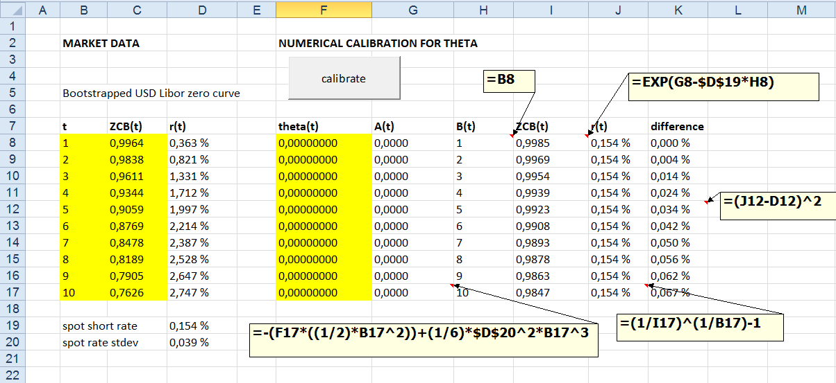
A few words concerning this worksheet. Zero-coupon bond curve maturities and prices are given in the columns B and C (yellow). Corresponding yields are calculated in the column D. Vector of time-dependent piecewise constant thetas will be calibrated and printed into column F (yellow). Columns from G to K are using analytical solution for Ho-Lee model to calculate theoretical zero-coupon bond prices and yields. Squared differences between market yields and calculated theoretical yields are given in the column K.

Input (output) data for (from) C# program are going to be read (written) directly from (to) Excel named ranges. Create the following named Excel ranges.

Finally, insert a new standard VBA module and create simple program calling the actual C# program (Sub tester). Also, create event-handling program for commandbutton click, which then calls the procedure shown below.

Concerning the program and its interfacing with Excel, all those small pieces have finally been assembled together. Now, it is time to do the actual calibration test run.

TEST RUN AND MODEL VALIDATION

In this section we will perform test run and check, whether our calibration model is working properly. In another words, are we able to replicate the market with our model. After pressing "calibrate" button, my Excel shows the following calibration results for theta parameters shown in column F.

Analytical results are already calculated in the worksheet (columns G to J). For example, time-dependent theta parameter for 4 years is 0.00771677. With this theta value embedded in A coefficient will produce zero-coupon bond price, equal to corresponding market price.

How about using SDE directly with these calibrated time-dependent thetas? Let us use Monte Carlo to price 4-year zero-coupon bond by using SDE directly. For the sake of simplicity, we perform this exercise in Excel. Simulation scheme is presented in the screenshot below.

In this Excel worksheet presented above, 4-year period has been divided into 800 time steps, which gives us the size for one time step to be 0.005 years. Total of 16 378 paths was simulated by using Ho-Lee SDE with calibrated time-dependent piecewise constant theta parameter. All simulated zero-coupon bond prices have been calculated in the row 805. By taking the average for all these 16 378 simulated zero-coupon bond prices, gives us the value of 0.9343. Needless to say this value is  random variable, which changes every time we press that F9 button. Our corresponding market price for 4-year zero-coupon bond is 0.9344, so we are not far away from that value. We can make the conclusion, that our calibration is working as expected.

Thanks for reading this blog.
-Mike