Python-QuantLib-SciPy: Optimizing Smooth Libor Forward Curve Revisited

One reader was making a remark, that my implementation for curve calibration scheme as presented in here, was not implemented by using QuantLib. As I was re-thinking my implementation, I suddenly remembered that in QuantLib, there are actually several ways to create yield term structures. One such approach is to create yield term structure from a set of given dates and forward rates. Also, VanillaSwap class gives us a direct mechanism for valuing swap transaction by using constructed curve. Bingo. So, this post is re-visiting curve calibration scheme, but this time implemented by using relevant QuantLib-Python library tools.

A few words about utility classes. Convert class will be used for transforming specific in-built data types into specific QuantLib types (Date, Calendar, DayCounter, etc). VanillaSwap class is just a wrapper for corresponding QuantLib.VanillaSwap class. It should be noted, that there is conventional NPV method for requesting swap PV by giving two specific arguments (yield term structure and floating leg index). There is also another method NPV_calibration, which is used for calculating swap PV during calibration process. For this method, input arguments are list of forward rates, list of forward dates and list of initial market rates. From this information, specific yield term structure implementation (QuantLib.ForwardCurve) will be created and used for valuing swap transaction.

import re
import numpy as np
import scipy.optimize as opt
import matplotlib.pyplot as pl
import QuantLib as ql

# utility class for different QuantLib type conversions 
class Convert():
    
    # convert date string ('yyyy-mm-dd') to QuantLib Date object
    def to_date(s):
        monthDictionary = {
            '01': ql.January, '02': ql.February, '03': ql.March,
            '04': ql.April, '05': ql.May, '06': ql.June,
            '07': ql.July, '08': ql.August, '09': ql.September,
            '10': ql.October, '11': ql.November, '12': ql.December
        }
        arr = re.findall(r"[\w']+", s)
        return ql.Date(int(arr[2]), monthDictionary[arr[1]], int(arr[0]))
    
    # convert string to QuantLib businessdayconvention enumerator
    def to_businessDayConvention(s):
        if (s.upper() == 'FOLLOWING'): return ql.Following
        if (s.upper() == 'MODIFIEDFOLLOWING'): return ql.ModifiedFollowing
        if (s.upper() == 'PRECEDING'): return ql.Preceding
        if (s.upper() == 'MODIFIEDPRECEDING'): return ql.ModifiedPreceding
        if (s.upper() == 'UNADJUSTED'): return ql.Unadjusted
        
    # convert string to QuantLib calendar object
    def to_calendar(s):
        if (s.upper() == 'TARGET'): return ql.TARGET()
        if (s.upper() == 'UNITEDSTATES'): return ql.UnitedStates()
        if (s.upper() == 'UNITEDKINGDOM'): return ql.UnitedKingdom()
        # TODO: add new calendar here
        
    # convert string to QuantLib swap type enumerator
    def to_swapType(s):
        if (s.upper() == 'PAYER'): return ql.VanillaSwap.Payer
        if (s.upper() == 'RECEIVER'): return ql.VanillaSwap.Receiver
        
    # convert string to QuantLib frequency enumerator
    def to_frequency(s):
        if (s.upper() == 'DAILY'): return ql.Daily
        if (s.upper() == 'WEEKLY'): return ql.Weekly
        if (s.upper() == 'MONTHLY'): return ql.Monthly
        if (s.upper() == 'QUARTERLY'): return ql.Quarterly
        if (s.upper() == 'SEMIANNUAL'): return ql.Semiannual
        if (s.upper() == 'ANNUAL'): return ql.Annual

    # convert string to QuantLib date generation rule enumerator
    def to_dateGenerationRule(s):
        if (s.upper() == 'BACKWARD'): return ql.DateGeneration.Backward
        if (s.upper() == 'FORWARD'): return ql.DateGeneration.Forward
        # TODO: add new date generation rule here

    # convert string to QuantLib day counter object
    def to_dayCounter(s):
        if (s.upper() == 'ACTUAL360'): return ql.Actual360()
        if (s.upper() == 'ACTUAL365FIXED'): return ql.Actual365Fixed()
        if (s.upper() == 'ACTUALACTUAL'): return ql.ActualActual()
        if (s.upper() == 'ACTUAL365NOLEAP'): return ql.Actual365NoLeap()
        if (s.upper() == 'BUSINESS252'): return ql.Business252()
        if (s.upper() == 'ONEDAYCOUNTER'): return ql.OneDayCounter()
        if (s.upper() == 'SIMPLEDAYCOUNTER'): return ql.SimpleDayCounter()
        if (s.upper() == 'THIRTY360'): return ql.Thirty360()
        
    # convert string (ex.'USDLibor.3M') to QuantLib ibor index object
    # note: forwarding term structure has to be linked to index object separately
    def to_iborIndex(s):
        s = s.split('.')
        if(s[0].upper() == 'USDLIBOR'): return ql.USDLibor(ql.Period(s[1]))
        if(s[0].upper() == 'EURIBOR'): return ql.Euribor(ql.Period(s[1]))  

class VanillaSwap(object):
    
    def __init__(self, ID, swapType, nominal, startDate, maturityDate, fixedLegFrequency, 
        fixedLegCalendar, fixedLegConvention, fixedLegDateGenerationRule, fixedLegRate, fixedLegDayCount,
        fixedLegEndOfMonth, floatingLegFrequency, floatingLegCalendar, floatingLegConvention, 
        floatingLegDateGenerationRule, floatingLegSpread, floatingLegDayCount, 
        floatingLegEndOfMonth, floatingLegIborIndex):

        # create member data, convert all required QuantLib types
        self.ID = str(ID)
        self.swapType = Convert.to_swapType(swapType)
        self.nominal = float(nominal)
        self.startDate = Convert.to_date(startDate)
        self.maturityDate = Convert.to_date(maturityDate)
        self.fixedLegFrequency = ql.Period(Convert.to_frequency(fixedLegFrequency))
        self.fixedLegCalendar = Convert.to_calendar(fixedLegCalendar)
        self.fixedLegConvention = Convert.to_businessDayConvention(fixedLegConvention)
        self.fixedLegDateGenerationRule = Convert.to_dateGenerationRule(fixedLegDateGenerationRule)
        self.fixedLegRate = float(fixedLegRate)
        self.fixedLegDayCount = Convert.to_dayCounter(fixedLegDayCount)
        self.fixedLegEndOfMonth = bool(fixedLegEndOfMonth)
        self.floatingLegFrequency = ql.Period(Convert.to_frequency(floatingLegFrequency))
        self.floatingLegCalendar = Convert.to_calendar(floatingLegCalendar)
        self.floatingLegConvention = Convert.to_businessDayConvention(floatingLegConvention)
        self.floatingLegDateGenerationRule = Convert.to_dateGenerationRule(floatingLegDateGenerationRule)
        self.floatingLegSpread = float(floatingLegSpread)
        self.floatingLegDayCount = Convert.to_dayCounter(floatingLegDayCount)
        self.floatingLegEndOfMonth = bool(floatingLegEndOfMonth)
        self.floatingLegIborIndex = Convert.to_iborIndex(floatingLegIborIndex)

        # create fixed leg schedule
        self.fixedLegSchedule = ql.Schedule(
            self.startDate, 
            self.maturityDate,
            self.fixedLegFrequency, 
            self.fixedLegCalendar, 
            self.fixedLegConvention,
            self.fixedLegConvention,
            self.fixedLegDateGenerationRule,
            self.fixedLegEndOfMonth)
        
        # create floating leg schedule
        self.floatingLegSchedule = ql.Schedule(
            self.startDate, 
            self.maturityDate,
            self.floatingLegFrequency, 
            self.floatingLegCalendar, 
            self.floatingLegConvention,
            self.floatingLegConvention,
            self.floatingLegDateGenerationRule,
            self.floatingLegEndOfMonth)

    # NPV method used for specific calibration purposes
    # x = list of forward rates
    # args: 0 = list of forward dates, 1 = list of market rates        
    def NPV_calibration(self, x, args):
        # concatenate given market rates and given forward rates
        x = np.concatenate([args[1], x])
        
        # create QuantLib yield term structure object
        # from a given set of forward rates and dates
        curve = ql.YieldTermStructureHandle(ql.ForwardCurve(args[0], x, 
            self.floatingLegDayCount, self.floatingLegCalendar))        

        # set forwarding term structure to floating leg index
        self.floatingLegIborIndex = self.floatingLegIborIndex.clone(curve) 
        
        # create vanilla interest rate swap
        self.instrument = ql.VanillaSwap(
            self.swapType, 
            self.nominal, 
            self.fixedLegSchedule, 
            self.fixedLegRate, 
            self.fixedLegDayCount, 
            self.floatingLegSchedule,
            self.floatingLegIborIndex,
            self.floatingLegSpread, 
            self.floatingLegDayCount)
        
        # pair instrument with pricing engine, request PV
        self.instrument.setPricingEngine(ql.DiscountingSwapEngine(curve))
        return self.instrument.NPV()
    
    # NPV method used for general pricing purposes
    def NPV(self, yieldTermStructureHandle, floatingLegIborIndex):
        # set forwarding term structure to floating leg index
        self.floatingLegIborIndex = floatingLegIborIndex.clone(yieldTermStructureHandle)
        
        # create vanilla interest rate swap
        self.instrument = ql.VanillaSwap(
            self.swapType, 
            self.nominal, 
            self.fixedLegSchedule, 
            self.fixedLegRate, 
            self.fixedLegDayCount, 
            self.floatingLegSchedule,
            self.floatingLegIborIndex,
            self.floatingLegSpread, 
            self.floatingLegDayCount)
        
        # pair instrument with pricing engine, request PV
        self.instrument.setPricingEngine(ql.DiscountingSwapEngine(yieldTermStructureHandle))
        return self.instrument.NPV()

ObjectiveFunction is used for minimization process for calculating sum of squared errors of all adjacent forward rates. Maximum smoothness of the curve will be achieved as a result of this minimization.

# objective function calculates sum of squared errors of all decision variables
# x = list of forward rates
# args: 0 = list of market rates data, 1 = scaling factor
def ObjectiveFunction(x, args):
    # concatenate given market rates and forward rates
    x = np.concatenate([args[0], x])
    return np.sum(np.power(np.diff(x), 2) * args[1])

The actual program flow will start by creating a set of vanilla interest rate swap objects (VanillaSwap) into list.

# dynamic data parts for set of vanilla swaps 
swapIDs = ['2Y', '3Y', '4Y', '5Y', '6Y', '7Y', '8Y', '9Y', '10Y', '12Y', '15Y', '20Y', '25Y', '30Y']
maturities = ['2010-02-08', '2011-02-07', '2012-02-06', '2013-02-06', '2014-02-06', '2015-02-06', '2016-02-08', 
    '2017-02-06', '2018-02-06', '2020-02-06', '2023-02-06', '2028-02-07', '2033-02-07', '2038-02-08']
swapRates = [0.02795, 0.03035, 0.03275, 0.03505, 0.03715, 0.03885, 0.04025, 0.04155, 0.04265, 0.04435, 
    0.04615, 0.04755, 0.04805, 0.04815]

# create vanilla swap transaction objects into list
swaps = [VanillaSwap(swapID, 'Payer', 1000000, '2008-02-06', maturity, 'Annual', 
    'Target', 'ModifiedFollowing', 'Backward', swapRate, 'Actual360', False, 'Quarterly', 
    'Target', 'ModifiedFollowing', 'Backward', 0.0, 'Actual360', False, 'USDLibor.3M')
    for swapID, maturity, swapRate in zip(swapIDs, maturities, swapRates)]

Next, the program will initialize the actual market data (to be used in forward curve), starting values for forward curve, set of dates for forward curve, optimization constraints and the actual optimization model.

# take initial forward rates from market data, set initial guesses and scaling factor for objective function
initialMarketData = np.array([0.03145, 0.0279275, 0.0253077, 0.0249374])
initialForwardGuesses = np.full(117, 0.02)
scalingFactor = 1000000.0

# create relevant QuantLib dates
today = ql.Date(4, 2, 2008)
ql.Settings.instance().evaluationDate = today  
settlementDate = ql.TARGET().advance(today, ql.Period(2, ql.Days))

# create set of dates for forward curve
dates = list(ql.Schedule(settlementDate, ql.Date(6, 2, 2038), ql.Period(ql.Quarterly), ql.TARGET(),
    ql.ModifiedFollowing, ql.ModifiedFollowing, ql.DateGeneration.Backward, False))

# create constraints for optimization model
swapConstraints = tuple([{'type': 'eq', 'fun': swap.NPV_calibration, 'args': [[dates, initialMarketData]]} for swap in swaps])

# create and execute scipy minimization model
model = opt.minimize(ObjectiveFunction, initialForwardGuesses, args = ([initialMarketData, scalingFactor]), 
    method = 'SLSQP', options = {'maxiter': 500}, constraints = swapConstraints)

After processing optimization model, the actual calibrated forward rates can be requested from the model. Next part of the program will just plot the calibrated forward term structure.

# extract calibrated forward rates, create times and plot term structure
forwards = np.concatenate([initialMarketData, model.x])
times = np.array([ql.Actual360().yearFraction(settlementDate, date) for date in dates])
pl.plot(times, forwards)
pl.show()

Final part of the program will create QuantLib yield term structure (QuantLib.ForwardCurve) and re-values our initial set of swap transactions. All swaps will be priced to zero at inception date.

# create new QuantLib curve from calibrated forward rates
curve = ql.YieldTermStructureHandle(ql.ForwardCurve(dates, forwards, ql.Actual360(), ql.TARGET()))

# value initial set of vanilla swaps using new QuantLib valuation curve
# all swaps will be priced to zero at inception date
for swap in swaps:
    index = ql.USDLibor(ql.Period(3, ql.Months), curve)
    pv = swap.NPV(curve, index)
    print(swap.ID, '{0:.5f}'.format(pv))

It should be noted, that by utilizing calibration scheme presented in this post, valuation curves (yield term structures) for QuantLib for all currencies and for all different basis can be constructed (assuming the relevant market data exists). Next logical step would be to implement similar scheme for calibrating valuation curves for QuantLib for cross-currency cases and within collateralized world.

Complete program can be downloaded from my GitHub page. Example data has been taken from chapter three within excellent book by Richard Flavell. Finally, thanks again for reading this blog.
-Mike

Python-SciPy: Optimizing Smooth Libor Forward Curve

In my previous post, I presented how to use Python SciPy Optimization package for solving zero-coupon rate term structure from a given set of zero-coupon bond prices numerically. In this post, the same approach will be used in order to solve smooth Libor forward curve from a given set of vanilla swaps. Example of applying this scheme using Solver and Excel/VBA can be found in here.

In order to value fixed income derivatives cash flows, relevant forward rates and discount factors have to be defined from bootstrapped zero-coupon curve. In a Libor world, we use cash and FRA contracts (or futures contracts) in a short-end of the curve, while in a long-end of the curve we use swap contracts. Let us assume for a moment, that we bootstrap USD 3M zero-coupon curve, in order to get 3M forward rates on a quarterly basis. While bootstrapping approach usually gives smooth curve within short-end of the curve, it will usually fail to do this within long-end of the curve. This happens, because there is no swap contracts available in a long-end of the curve and hereby, we need to do a lot of interpolations for required swap rates. The resulting forward curve then looks like a chain of waterfalls and for the long-end of the curve, smoothness will be lost. This topic has been thoroughly covered in chapter three within this excellent book by Richard Flavell.

In a nutshell, we first define the shortest end of the curve (using spot cash rate) and then we just guess the rest of the forward rates. After this, we minimize sum of squared differences between adjacent forward rates, subject to constraints. In this case, constraints are present values of swaps, which by definition will be zero. When this optimization task has been performed, the resulting forward curve will successfully re-price the current swap market.

Bloomberg forward curve screen for the same set of data is available in here. Finally, thanks again for reading my blog.
-Mike

import numpy as np
import scipy.optimize as opt
import matplotlib.pyplot as pl

# sum of squared errors of all decision variables
# args: 0 = array of given initial rates, 1 = scaling factor
def ObjectiveFunction(x, args):
    # concatenate given initial rates and given 'guesses' for forward rates
    x = np.concatenate([args[0], x])
    return np.sum(np.power(np.diff(x), 2) * args[1])

# x = array of Libor forward rates
# args: 0 = swap rate, 1 = years to maturity, 2 = floating leg payments per year, 
# 3 = notional, 4 = array of given initial rates
def VanillaSwapPV(x, args):
    # PV (fixed payer swap) = -swapRate * Q(T) + (1 - DF(T))
    # where Q(T) is sumproduct of fixed leg discount factors and corresponding time accrual factors
    # assumption : fixed leg is always paid annually
    # since fixed leg is paid annually and maturity is always integer, 
    # time accrual factor will always be exactly 1.0
    
    # concatenate given initial rates and given 'guesses' for forward rates
    x = np.concatenate([args[4], x])
    DF = 0.0
    Q  = 0.0
    floatingLegTenor = 1 / args[2]
    nextFixedLegCouponDate = 1
    currentTimePoint = 0.0
    nCashFlows = int(args[1] * args[2])
    
    for i in range(nCashFlows):
        currentTimePoint += floatingLegTenor
        # first rate is always spot rate: calculate first spot discount factor
        if (i == 0):
            DF = 1 / (1 + x[i] * floatingLegTenor)
        # other rates are always forward rates
        if (i > 0):
            # solve current spot discount factor using previous spot discount factor
            # and current forward discount factor: DF(0,T) = DF(0,t) * DF(t,T), where (0 < t < T)
            DF *= (1 / (1 + x[i] * floatingLegTenor))
            if ((currentTimePoint - nextFixedLegCouponDate) == 0):
                Q += DF
                nextFixedLegCouponDate += 1
                
    return (-args[0] * Q + (1.0 - DF)) * args[3]

# array of given initial rates (the first given rate has to be spot cash rate)
# here, we give only one: 3M spot Libor fixing rate ('cash-to-first-future')
initialRates = np.array([0.006276])
scalingFactor = 1000000.0

# vanilla swap pricing functions as constraints
# args: swapRate, yearsToMaturity, floatingLegPaymentFrequency, notional, array of given initial rates
swaps = ({'type': 'eq', 'fun': VanillaSwapPV, 'args': [[0.0078775, 1, 4, scalingFactor, initialRates]]},
        {'type': 'eq', 'fun': VanillaSwapPV, 'args': [[0.009295, 2, 4, scalingFactor, initialRates]]},
        {'type': 'eq', 'fun': VanillaSwapPV, 'args': [[0.0103975, 3, 4, scalingFactor, initialRates]]},
        {'type': 'eq', 'fun': VanillaSwapPV, 'args': [[0.01136, 4, 4, scalingFactor, initialRates]]},
        {'type': 'eq', 'fun': VanillaSwapPV, 'args': [[0.012268, 5, 4, scalingFactor, initialRates]]},
        {'type': 'eq', 'fun': VanillaSwapPV, 'args': [[0.013183, 6, 4, scalingFactor, initialRates]]},
        {'type': 'eq', 'fun': VanillaSwapPV, 'args': [[0.01404, 7, 4, scalingFactor, initialRates]]},
        {'type': 'eq', 'fun': VanillaSwapPV, 'args': [[0.014829, 8, 4, scalingFactor, initialRates]]},
        {'type': 'eq', 'fun': VanillaSwapPV, 'args': [[0.01554, 9, 4, scalingFactor, initialRates]]},
        {'type': 'eq', 'fun': VanillaSwapPV, 'args': [[0.016197, 10, 4, scalingFactor, initialRates]]},
        {'type': 'eq', 'fun': VanillaSwapPV, 'args': [[0.016815, 11, 4, scalingFactor, initialRates]]},
        {'type': 'eq', 'fun': VanillaSwapPV, 'args': [[0.017367, 12, 4, scalingFactor, initialRates]]},
        {'type': 'eq', 'fun': VanillaSwapPV, 'args': [[0.018645, 15, 4, scalingFactor, initialRates]]},
        {'type': 'eq', 'fun': VanillaSwapPV, 'args': [[0.01996, 20, 4, scalingFactor, initialRates]]},
        {'type': 'eq', 'fun': VanillaSwapPV, 'args': [[0.020615, 25, 4, scalingFactor, initialRates]]},
        {'type': 'eq', 'fun': VanillaSwapPV, 'args': [[0.02097, 30, 4, scalingFactor, initialRates]]},
        {'type': 'eq', 'fun': VanillaSwapPV, 'args': [[0.021155, 40, 4, scalingFactor, initialRates]]},
        {'type': 'eq', 'fun': VanillaSwapPV, 'args': [[0.021017, 50, 4, scalingFactor, initialRates]]})

# initial guesses for Libor forward rates up to 50 years
# number of rates: 50 * 4 - 1 (years to maturity * floating leg payments per year - first given cash spot rate)
initialGuesses = np.full(199, 0.006)
model = opt.minimize(ObjectiveFunction, initialGuesses, args = ([initialRates, scalingFactor]), method = 'SLSQP', options = {'maxiter': 500}, constraints = swaps)

# print selected model results
print('Success: ' + str(model.success))
print('Message: ' + str(model.message))
print('Number of iterations: ' + str(model.nit))
print('Objective function (sum of squared errors): ' + str(model.fun))
#print('Changing variables (Libor forward rates): ' + str(model.x * 100))
pl.plot(model.x)
pl.show()

Python-SciPy: Solving Zero-Coupon Term Structure Using Optimization

This post is presenting how to use Python SciPy Optimization package for solving out zero-coupon rate term structure from a given set of zero-coupon bond prices. Needless to say, we do not need any numerical method to do this, since we have exact analytical formulas for backing out zero-coupon rates from zero-coupon bond prices. However, approach presented in this relatively simple example can be applied into more interesting schemes, such as solving out smooth Libor forward curve from a given set of vanilla swaps. Example of such scheme using Solver and Excel/VBA can be found in here.

Let us assume zero-coupon rate term structure as shown below. Let us also assume, that the only information we can observe is the zero-coupon bond prices. Our task is to solve zero-coupon rates term structure.

In a nutshell, we first set initial guesses for ten zero-coupon rates. After this we minimize sum of squared differences between adjacent zero-coupon rates (in objective function), but subject to constraints. In this case, constraints are differences between observed zero-coupon bond market prices and calculated bond prices, which need to be pushed to zero. When this optimization task has been completed, the resulting zero-coupon term structure will successfully re-price the current zero-coupon bond market, while curve smoothness is maximized. Example program results are shown below.

Thanks for reading this blog.
-Mike

import numpy as np
import scipy.optimize as opt
import matplotlib.pyplot as pl

# sum of squared errors of decision variables
def ObjectiveFunction(x, args):
    return np.sum(np.power(np.diff(x), 2) * args[0])

# zero coupon bond pricing function
def ZeroCouponBond(x, args):
    # return difference between calculated and market price
    return ((1 / (1 + x[args[3]])**args[2]) - args[0]) * args[1]

# zero coupon bond pricing functions as constraints
# args: market price, scaling factor, maturity, index number for rate array
zeroPrices = ({'type': 'eq', 'fun': ZeroCouponBond, 'args': [[0.998801438274071, 1000000.0, 1.0, 0]]},
            {'type': 'eq', 'fun': ZeroCouponBond, 'args': [[0.996210802629012, 1000000.0, 2.0, 1]]},
            {'type': 'eq', 'fun': ZeroCouponBond, 'args': [[0.991943543964159, 1000000.0, 3.0, 2]]},
            {'type': 'eq', 'fun': ZeroCouponBond, 'args': [[0.981028206597786, 1000000.0, 4.0, 3]]},
            {'type': 'eq', 'fun': ZeroCouponBond, 'args': [[0.962851266220459, 1000000.0, 5.0, 4]]},
            {'type': 'eq', 'fun': ZeroCouponBond, 'args': [[0.946534719794057, 1000000.0, 6.0, 5]]},
            {'type': 'eq', 'fun': ZeroCouponBond, 'args': [[0.924997530805076, 1000000.0, 7.0, 6]]},
            {'type': 'eq', 'fun': ZeroCouponBond, 'args': [[0.912584111300984, 1000000.0, 8.0, 7]]},
            {'type': 'eq', 'fun': ZeroCouponBond, 'args': [[0.892632531026722, 1000000.0, 9.0, 8]]},
            {'type': 'eq', 'fun': ZeroCouponBond, 'args': [[0.877098137542374, 1000000.0, 10.0, 9]]})

# initial guesses for ten zero-coupon rates
initialGuess = np.full(10, 0.005)
model = opt.minimize(ObjectiveFunction, initialGuess, args = ([1000000.0]), method = 'SLSQP', constraints = zeroPrices)

# print selected model results
print('Success: ' + str(model.success))
print('Message: ' + str(model.message))
print('Number of iterations: ' + str(model.nit))
print('Objective function (sum of squared errors): ' + str(model.fun))
print('Changing variables (zero-coupon rates): ' + str(model.x * 100))
pl.plot(model.x)
pl.show()

Excel/VBA : Optimizing smooth OIS-adjusted Libor forward curve using Solver

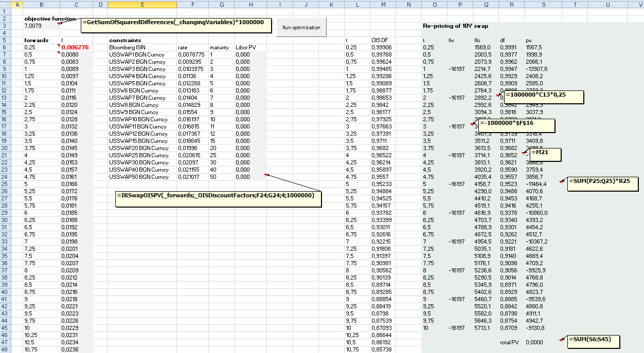
Optimization for Libor forward curve has been presented in this blog post. This time, we will adjust the presented optimization procedure in such way, that OIS-adjusted Libor forward rates are going to be solved for a given fixed set of swap rates and OIS discount factors.

In a nutshell, justification for OIS-adjusted forward rates is the following :

• In the "old world", we first bootstrapped Libor zero-coupon curve, from which we calculated Libor discount factors and Libor forward rates (for constructing floating leg coupons) at the same time. Only one curve was ever needed to accomplish this procedure. 
• In the "new world", since all swap cash flows are discounted using OIS discount factors and par swap rates are still used for constructing swap fixed leg cash flows, forward rates (OIS-adjusted Libor forward rates) have to be slightly adjusted, in order to equate present value of all swap cash flows back to be zero.

All the relevant issues have been clearly explained in this research paper by Barclays.

Screenshots below are showing required Excel worksheet setups along with optimized OIS-adjusted Libor forward curve and required additions to existing VBA program needed to perform this optimization task. In order to validate the optimized OIS-adjusted Libor forward curve, a 10-year vanilla swap has been re-priced using optimized OIS-adjusted Libor forward rates and given set of fixed OIS discount factors.

When setting up VBA program, first implement the program presented in this blog post. After this, add two new functions (IRSwapOISPV, linearInterpolation) presented below into module XLSFunctions. Finally, remember to include references to Solver and Microsoft Scripting Runtime libraries.

Thanks for reading this blog.
-Mike

Public Function IRSwapOISPV(ByRef forwards As Excel.Range, ByRef OISDF As Excel.Range, ByVal swapRate As Double, _
ByVal yearsToMaturity As Integer, ByVal floatingLegPaymentFrequency As Integer, ByVal notional As Double) As Double
    '
    ' PV (fixed payer swap) = -swapRate * Q_fixed + Q_float
    ' where Q_fixed is sumproduct of fixed leg OIS discount factors and corresponding time accrual factors
    ' and Q_float is sumproduct of adjusted libor forward rates, OIS discount factors and corresponding time accrual factors
    ' assumption : fixed leg is always paid annually
    ' since fixed leg is paid annually and maturity is always integer, time accrual factor will always be exactly 1.0
    Dim f As Variant: f = forwards.Value2
    Dim DF As Variant: DF = OISDF.Value2
    Dim Q_fixed As Double
    Dim Q_float As Double
    Dim floatingLegTenor As Double: floatingLegTenor = 1 / CDbl(floatingLegPaymentFrequency)
    Dim nextFixedLegCouponDate As Integer: nextFixedLegCouponDate = 1
    Dim currentTimePoint As Double: currentTimePoint = CDbl(0)
    '
    Dim i As Integer
    For i = 1 To (yearsToMaturity * floatingLegPaymentFrequency)
        currentTimePoint = currentTimePoint + floatingLegTenor
        '
        ' update floating leg Q
        Q_float = Q_float + f(i, 1) * linearInterpolation(currentTimePoint, OISDF.Value2) * floatingLegTenor
        '
        ' update fixed leg Q, if current time point is coupon payment date
        If ((currentTimePoint - CDbl(nextFixedLegCouponDate)) = 0) Then
            Q_fixed = Q_fixed + linearInterpolation(currentTimePoint, OISDF.Value2)
            nextFixedLegCouponDate = nextFixedLegCouponDate + 1
        End If
    Next i
    IRSwapOISPV = (-swapRate * Q_fixed + Q_float) * notional
End Function
'
Public Function linearInterpolation(ByVal maturity As Double, ByRef curve As Variant) As Double
    '
    ' read range into Nx2 array
    Dim r As Variant: r = curve
    '
    Dim n As Integer: n = UBound(r, 1)
    '
    ' boundary checkings
    If ((r(LBound(r, 1), 1)) > maturity) Then linearInterpolation = r(LBound(r, 1), 2): Exit Function
    If ((r(UBound(r, 1), 1)) < maturity) Then linearInterpolation = r(UBound(r, 1), 2): Exit Function
    '
    Dim i As Long
    For i = 1 To n
        If ((r(i, 1) <= maturity) And (r(i + 1, 1) >= maturity)) Then
            '
            Dim y0 As Double: y0 = r(i, 2)
            Dim y1 As Double: y1 = r(i + 1, 2)
            Dim x0 As Double: x0 = r(i, 1)
            Dim x1 As Double: x1 = r(i + 1, 1)
            '
            linearInterpolation = y0 + (y1 - y0) * ((maturity - x0) / (x1 - x0))
            Exit For
        End If
    Next i
End Function
'

Excel/VBA : Optimizing smooth Libor forward curve using Solver

In order to value fixed income derivatives cash flows, relevant forward rates and discount factors have to be defined from bootstrapped zero-coupon curve. In a Libor world, we use cash and FRA contracts (or futures contracts) in a short-end of the curve, while in a long-end of the curve we use relevant swap contracts. Let us assume for a moment, that we bootstrap zero-coupon curve, in order to define those forward rates and discount factors on a quarterly basis. While bootstrapping usually gives a smooth curve for a short-end of the curve, it will usually fail to do this for a long-end of the curve. This happens, because there is no relevant swap contracts available in a long-end of the curve and hereby, we need to do a lot of interpolation in a long-end of the curve for swaps. The resulting forward curve then looks like a chain of waterfalls.

This time, I wanted to present a cool way to solve those forward rates by using numerical optimization scheme. The topic itself has been thoroughly covered in chapter three in excellent book by Richard Flavell. In a nutshell, we first define the shortest end of the curve (using cash and forwards) and then we just guess the rest of the forward rates. After this, we minimize sum of squared differences between adjacent forward rates, subject to constraints. In this case, constraints are present values of swaps, which by definition will be zero. When this optimization task has been performed, the resulting forward curve will successfully re-price the current swap market.

In Excel worksheet, there has to be three named ranges to be used by VBA program:

• Objective function (sum of squared differences between adjacent forward rates)
• Constraints (swap PV for each swap contract used)
• Decision variables (forward rates to be solved)

Screenshots below are showing required Excel worksheet setups along with optimized Libor forward curve, corresponding capture of Bloomberg smoothed forward curve and the actual VBA program needed to perform optimization task. Note, that for this example, I have been defining only the first 3-month Libor spot rate fixing. The rest of the forward rates are going to be solved. When setting up VBA program, remember to include references to Solver and Microsoft Scripting Runtime libraries.

Finally, thanks for reading my blog.
-Mike

' Worksheet : Libor
Option Explicit
'
Private Sub btnSolveLibor_Click()
    '
    ' define Excel ranges for objective function, decision variables and constraints
    Dim objectiveFunction As Range: Set objectiveFunction = Range("_objectiveFunction")
    Dim changingVariables As Range: Set changingVariables = Range("_changingVariables")
    Dim constraints As Range: Set constraints = Range("_constraints")
    '
    ' create parameter wrapper
    ' for objective function, decision variables and constraints, address of range is needed
    Dim parameters As New Scripting.Dictionary
    parameters.Add PRM.objectiveFunction, CStr(objectiveFunction.Address)
    parameters.Add PRM.changingVariables, CStr(changingVariables.Address)
    parameters.Add PRM.constraints, CStr(constraints.Address)
    parameters.Add PRM.maxMinVal, CInt(2) ' max=1, min=2, valueof=3
    parameters.Add PRM.userFinish, CBool(True)
    parameters.Add PRM.assumeNonNegative, CBool(False)
    parameters.Add PRM.relation, CInt(2) ' lessOrEqual=1, equal=2, greaterOrEqual=3
    parameters.Add PRM.formulaText, CStr("0.0")
    '
    ' create instance of constrained optimization model implementation
    Dim xlSolver As ISolver: Set xlSolver = New ConstrainedOptimization
    xlSolver.solve parameters
    '
    ' release objects
    Set xlSolver = Nothing
    Set parameters = Nothing
End Sub
'
'
'
'
'
' Module : Enumerators
Option Explicit
'
' enumerator needed for parameter wrapper
Public Enum PRM
    objectiveFunction = 1
    maxMinVal = 2
    valueOf = 3
    changingVariables = 4
    userFinish = 5
    assumeNonNegative = 6
    constraints = 7
    relation = 8
    formulaText = 9
End Enum
'
'
'
'
'
' Module : XLSFunctions
Option Explicit
'
Public Function GetSumOfSquaredDifferences(ByRef values As Excel.Range) As Double
    '
    Dim v As Variant: v = values.Value2
    Dim sumOfSquaredDifferences As Double
    Dim i As Integer
    '
    ' calculate sum of squared differences between all adjacent values
    For i = 1 To (UBound(v) - 1)
        sumOfSquaredDifferences = sumOfSquaredDifferences + ((v(i + 1, 1) - v(i, 1)) * (v(i + 1, 1) - v(i, 1)))
    Next i
    GetSumOfSquaredDifferences = sumOfSquaredDifferences
End Function
'
Public Function IRSwapLiborPV(ByRef forwards As Excel.Range, ByVal swapRate As Double, _
ByVal yearsToMaturity As Integer, ByVal floatingLegPaymentFrequency As Integer, ByVal notional As Double) As Double
    '
    ' PV (fixed payer swap) = -swapRate * Q(T) + (1 - DF(T))
    ' where Q(T) is sumproduct of fixed leg discount factors and corresponding time accrual factors
    ' assumption : fixed leg is always paid annually
    ' since fixed leg is paid annually and maturity is always integer, time accrual factor will always be exactly 1.0
    Dim f As Variant: f = forwards.Value2
    Dim DF As Double
    Dim Q As Double
    Dim floatingLegTenor As Double: floatingLegTenor = 1 / CDbl(floatingLegPaymentFrequency)
    Dim nextFixedLegCouponDate As Integer: nextFixedLegCouponDate = 1
    Dim currentTimePoint As Double: currentTimePoint = CDbl(0)
    '
    Dim i As Integer
    For i = 1 To (yearsToMaturity * floatingLegPaymentFrequency)
        '
        currentTimePoint = currentTimePoint + floatingLegTenor
        ' first rate is always spot rate, calculate first spot discount factor
        If (i = 1) Then
            DF = 1 / (1 + f(i, 1) * floatingLegTenor)
        End If
        '
        ' other rates are always forward rates
        If (i > 1) Then
            ' solve current spot discount factor using previous spot discount factor
            ' and current forward discount factor : DF(0,2) = DF(0,1) * DF(1,2)
            DF = DF * (1 / (1 + f(i, 1) * floatingLegTenor))
            If ((currentTimePoint - CDbl(nextFixedLegCouponDate)) = 0) Then
                Q = Q + DF
                nextFixedLegCouponDate = nextFixedLegCouponDate + 1
            End If
        End If
    Next i
    IRSwapLiborPV = (-swapRate * Q + (1 - DF)) * notional
End Function
'
'
'
'
'
' Class module : ISolver
Option Explicit
'
' ISolver interface to be implemented
Public Function solve(ByRef parameters As Scripting.Dictionary)
    ' no implementation
End Function
'
'
'
'
'
' Class module : ConstrainedOptimization
Option Explicit
'
Implements ISolver
'
' implementation for ISolver interface
' solver model for constrained optimization tasks
Private Function ISolver_solve(ByRef parameters As Scripting.Dictionary)
    '
    ' reset solver model
    solver.SolverReset
    '
    ' create optimization task
    solver.SolverOk _
        parameters.Item(PRM.objectiveFunction), _
        parameters.Item(PRM.maxMinVal), _
        parameters.Item(PRM.valueOf), _
        parameters.Item(PRM.changingVariables)
    '
    ' add constraints
    solver.SolverAdd _
        parameters(PRM.constraints), _
        parameters(PRM.relation), _
        parameters(PRM.formulaText)
    '
    ' solve optimization model
    solver.SolverOptions AssumeNonNeg:=parameters.Item(PRM.assumeNonNegative)
    solver.SolverSolve parameters.Item(PRM.userFinish)
End Function
'