QuantLib-Python: Monte Carlo Valuation for Power Reverse Dual-Currency Note (PRDC)

PRDC note

Essentially, PRDC note can be thought as taking a leveraged position on FX forward curve. Floating coupon rate is a function of FX rates, usually defined as follows.

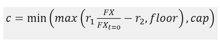
Additional FX term (at t=0) will scale FX rate used in coupon and is usually set to be equal to FX forward at inception. Mathematically, this changes the slope of coupon payoff and therefore, adding desired leverage to the product.

Model for FX stochastics

From pricing perspective, we need to get a view on FX forward curve. This can be simulated by using Garman-KohlHagen stochastic process for an exchange rate, which is available in QuantLib-Python library. In essence, this process is Geometric Brownian Motion, with an added term for foreign interest rate. We will use this model, even it does not necessarily fully reflect the statistical properties of exchange rate.

Applying Ito's rule to Geometric Brownian Motion, gives us the following solution for an exchange rate S observed at time t.

Python program

In order to implement completely new instrument and corresponding new pricing engine in QuantLib, one should first implement these in QuantLib C++ library by following carefully the designed Instrument-Engine scheme and then, interface these newly created C++ types back to Python by using swig. However in here, we will skip the previous approach completely. Instead, we just take "all the useful bits and pieces" available in QuantLib-Python library and use these to implement our own valuation code.

QuantLib-Python object building documentation by David Duarte is available in here.

The complete code is available in here.

Libraries

The following two libraries are being used.

import numpy as np import QuantLib as ql

FX path generator

Path generator implements spot rate simulation, based on a given 1D stochastic process. Generated path is exactly in line with the dates given in coupon schedule. Note, that the exact number of paths to be generated has not been defined in this class. Whoever will be the client for this class, can request as many paths as desired. 

class PathGenerator:
    def __init__(self, valuation_date, coupon_schedule, day_counter, process):        
        self.valuation_date = valuation_date
        self.coupon_schedule = coupon_schedule
        self.day_counter = day_counter
        self.process = process
        #
        self.create_time_grids()
        
    def create_time_grids(self):
        all_coupon_dates = np.array(self.coupon_schedule)
        remaining_coupon_dates = all_coupon_dates[all_coupon_dates > self.valuation_date]
        self.time_grid = np.array([self.day_counter.yearFraction(self.valuation_date, date) 
            for date in remaining_coupon_dates])
        self.time_grid = np.concatenate((np.array([0.0]), self.time_grid))
        self.grid_steps = np.diff(self.time_grid)
        self.n_steps = self.grid_steps.shape[0]
        
    def next_path(self):
        e = np.random.normal(0.0, 1.0, self.n_steps)
        spot = self.process.x0()
        dw = e * self.grid_steps
        path = np.zeros(self.n_steps, dtype=float)
        
        for i in range(self.n_steps):
            dt = self.grid_steps[i]
            t = self.time_grid[i]
            spot = self.process.evolve(t, spot, dt, dw[i])
            path[i] = spot

        return path

Monte Carlo pricer

Monte Carlo pricer class will use path generator for simulating requested number of FX paths. A call for method npv will trigger coupon rates simulation. Simulated rates will then be corrected by taking into account of intro coupon. Finally, a series of cash flows will be created, based on calculated coupon rates and schedule dates.

class MonteCarloPricerPRDC: def __init__(self, valuation_date, coupon_schedule, day_counter, notional, discount_curve_handle, payoff_function, fx_path_generator, n_paths, intro_coupon_schedule, intro_coupon_rate): self.valuation_date = valuation_date self.coupon_schedule = coupon_schedule self.day_counter = day_counter self.notional = notional self.discount_curve_handle = discount_curve_handle self.payoff_function = payoff_function self.fx_path_generator = fx_path_generator self.n_paths = n_paths self.intro_coupon_schedule = intro_coupon_schedule self.intro_coupon_rate = intro_coupon_rate # self.create_coupon_dates() def create_coupon_dates(self): self.all_coupon_dates = np.array(self.coupon_schedule) self.past_coupon_dates = self.all_coupon_dates[self.all_coupon_dates < self.valuation_date] n_past_coupon_dates = self.past_coupon_dates.shape[0] - 1 self.past_coupon_rates = np.full(n_past_coupon_dates, 0.0, dtype=float) self.remaining_coupon_dates = self.all_coupon_dates[self.all_coupon_dates > self.valuation_date] self.time_grid = np.array([self.day_counter.yearFraction(self.valuation_date, date) for date in self.remaining_coupon_dates]) self.grid_steps = np.concatenate((np.array([self.time_grid[0]]), np.diff(self.time_grid))) self.n_steps = self.grid_steps.shape[0] if(self.intro_coupon_schedule==None): self.has_intro_coupon = False else: self.intro_coupon_dates = np.array(self.intro_coupon_schedule) self.remaining_intro_coupon_dates = self.intro_coupon_dates[self.intro_coupon_dates > self.valuation_date] self.n_remaining_intro_coupon_dates = self.remaining_intro_coupon_dates.shape[0] if(self.n_remaining_intro_coupon_dates > 0): self.has_intro_coupon = True else: self.has_intro_coupon = False def simulate_coupon_rates(self): self.simulated_coupon_rates = np.zeros(self.n_steps, dtype=float) for i in range(self.n_paths): path = self.fx_path_generator.next_path() for j in range(self.n_steps): self.simulated_coupon_rates[j] += self.payoff_function(path[j]) self.simulated_coupon_rates = self.simulated_coupon_rates / self.n_paths if(self.has_intro_coupon): self.append_intro_coupon_rates() self.coupon_rates = np.concatenate((self.past_coupon_rates, self.simulated_coupon_rates)) self.n_coupon_cash_flows = self.coupon_rates.shape[0] def append_intro_coupon_rates(self): for i in range(self.n_remaining_intro_coupon_dates): self.simulated_coupon_rates[i] = self.intro_coupon_rate def create_cash_flows(self): self.coupon_cash_flows = np.empty(self.n_coupon_cash_flows, dtype=ql.FixedRateCoupon) for i in range(self.n_coupon_cash_flows): self.coupon_cash_flows[i] = ql.FixedRateCoupon(self.all_coupon_dates[i+1], self.notional, self.coupon_rates[i], self.day_counter, self.all_coupon_dates[i], self.all_coupon_dates[i+1]) self.coupon_leg = ql.Leg(self.coupon_cash_flows) redemption = ql.Redemption(self.notional, self.all_coupon_dates[-1]) self.redemption_leg = ql.Leg(np.array([redemption])) def npv(self): self.simulate_coupon_rates() self.create_cash_flows() self.redemption_leg_npv = ql.CashFlows.npv(self.redemption_leg, self.discount_curve_handle, False) self.coupon_leg_npv = ql.CashFlows.npv(self.coupon_leg, self.discount_curve_handle, False) date = [payment.date() for payment in self.coupon_leg] amount = [payment.amount() for payment in self.coupon_leg] amount[-1] += self.notional pv = [ql.CashFlows.npv(np.array([payment]), self.discount_curve_handle, False) for payment in self.coupon_leg] pv[-1] += self.redemption_leg_npv self.cash_flow_table = np.array([date, amount, pv]) return self.coupon_leg_npv + self.redemption_leg_npv

Hard-coded factory

The creation of Garman-Kohlhagen process is isolated into hard-coded factory method. In here, we just use flat forward curves and non-calibrated short rate models for the sake of simplicity. For more realistic creation of the curves and model calibrations, check out this and this.

def process_factory():
    today = ql.Settings.instance().evaluationDate
    
    domestic_curve = ql.FlatForward(today, ql.QuoteHandle(ql.SimpleQuote(0.01)), ql.Actual360())
    domestic_curve = ql.YieldTermStructureHandle(domestic_curve)
    foreign_curve = ql.FlatForward(today, ql.QuoteHandle(ql.SimpleQuote(0.03)), ql.Actual360())
    foreign_curve = ql.YieldTermStructureHandle(foreign_curve)
    
    fx_vol = ql.QuoteHandle(ql.SimpleQuote(0.1))
    fx_vol_curve = ql.BlackVolTermStructureHandle(ql.BlackConstantVol(today, ql.NullCalendar(), fx_vol, ql.Actual360()))    
    fx_spot = ql.QuoteHandle(ql.SimpleQuote(133.2681))
    
    return ql.GarmanKohlagenProcess(fx_spot, foreign_curve, domestic_curve, fx_vol_curve)

Main program

Main program creates all required components (JPY discount curve, process, schedules, generator and pricer) and then requests npv and cash flow table as Numpy ndarray (indexing: [0] = coupon dates, [1] = cash flows, [2] = present values of cash flows).

today = ql.Date(11, 4, 2023)
ql.Settings.instance().evaluationDate = today

# create JPY discount curve
discount_curve = ql.FlatForward(today, ql.QuoteHandle(ql.SimpleQuote(0.005)), ql.Actual360())
discount_curve_handle = ql.YieldTermStructureHandle(discount_curve)

# create FX process
process = process_factory()

# create schedules for coupon- and intro coupon payments
effectiveDate = ql.Date(3, ql.September, 2015)
terminationDate = ql.Date(3, ql.September, 2041)
coupon_schedule = ql.MakeSchedule(effectiveDate, terminationDate, ql.Period(6, ql.Months), 
    backwards=True, calendar=ql.TARGET(), convention=ql.ModifiedFollowing)

intro_coupon_termination_date = ql.Date(3, ql.September, 2016)
intro_coupon_schedule = ql.MakeSchedule(effectiveDate, intro_coupon_termination_date, ql.Period(6, ql.Months), 
    backwards=True, calendar=ql.TARGET(), convention=ql.ModifiedFollowing)

# create FX path generator
fx_path_generator = PathGenerator(today, coupon_schedule, ql.Actual360(), process)

# create PRDC pricer
notional = 300000000.0
intro_coupon_rate = 0.022
n_paths = 10000
prdc_payoff_function = lambda fx_rate : min(max(0.122 * (fx_rate / 120.0) - 0.1, 0.0), 0.022)
prdc_pricer = MonteCarloPricerPRDC(ql.Settings.instance().evaluationDate, coupon_schedule, ql.Actual360(),notional, 
    discount_curve_handle, prdc_payoff_function, fx_path_generator, n_paths, intro_coupon_schedule, intro_coupon_rate)

# request results
npv_ccy = prdc_pricer.npv()
print('PV in CCY: {}'.format(npv_ccy))
jpy_eur = 145.3275
npv_eur = npv_ccy / jpy_eur
print('PV in EUR: {}'.format(npv_eur))
print()
print('Cash flow dates: {}'.format(prdc_pricer.cash_flow_table[0]))
print()
print('Cash flows: {}'.format(prdc_pricer.cash_flow_table[1]))
print()
print('Present values of cash flows: {}'.format(prdc_pricer.cash_flow_table[2]))

Thanks for reading this blog.

-Mike

Python: Simulating Exposures Using Multiprocessing Pool

This post is presenting a scheme for simulating exposures for European call option on a non-dividend-paying stock by using Multiprocessing.Pool class (note: in Linux). There are several different options available when stepping into multiprocessing world, but for this specific purpose, Multiprocessing.Pool is robust enough. In a nutshell, we need to simulate a path for the underlying equity price and then calculate call option present value for each point in time. Complete program can be downloaded from my github.

Library imports

import multiprocessing as mp
import numpy as np
import scipy.stats as sc
import matplotlib.pyplot as pl
import time, math

Methods

# black scholes valuation of call option on non-dividend-paying equity
def VanillaCall(s, x, t, r, v):
    pv = 0.0
    # option value at maturity
    if((t - 0.0) < (1 / 365)):
        pv = max(s - x, 0.0)
    # option value before its maturity
    else:
        d1 = (math.log(s / x) + (r + 0.5 * v ** 2) * t) / (v * math.sqrt(t))
        d2 = (math.log(s / x) + (r - 0.5 * v ** 2) * t) / (v * math.sqrt(t))
        pv = (s * sc.norm.cdf(d1, 0.0, 1.0) - x * math.exp(-r * t) * sc.norm.cdf(d2, 0.0, 1.0))
    return pv

# globalize local parameters
def Globalizer(local_parameters):
    global global_parameters
    global_parameters = local_parameters

# simulate exposures by using
# - a given one-factor process (func_process)
# - a given pricing function (func_pricing)
def SimulateExposures(arg):
    # seed random number generator
    np.random.seed(arg)
    # unzip globalized tuple
    n_paths_per_process, n_steps, t, s_0, r, vol, func_pricing, func_process = global_parameters
    s = 0.0
    pv = 0.0
    dt = (t / n_steps)
    # create container for results
    paths = np.zeros(shape=(n_paths_per_process, n_steps + 1), dtype=float)
    for i in range(n_paths_per_process):
        s = s_0
        t_expiry = t
        # value product at path inception
        paths[i, 0] = func_pricing(s, t_expiry)
        # create array of normal random variates
        e = np.random.standard_normal(n_steps)
        for j in range(n_steps):
            s = func_process(s, e[j])
            t_expiry = (t - dt * (j + 1))
            # value product at after inception
            paths[i, j + 1] = func_pricing(s, t_expiry)
    return paths

Main program

The main program will create a pool containing two processes, which will use SimulateExposures method for calculating exposures for a call option. Method takes only random seed as its direct input argument. All the other required arguments (product- or process-related parameters) will be packed into tuple data structure, which will be globalized for each process separately in initializer method. After processing, the both worker methods will return an array of simulated exposures, which then will be aggregated into array (exposures).

t_0 = time.time()

# monte carlo parameters
n_paths = 10000
n_steps = 250
n_processes = 2
n_paths_per_process = int(n_paths / n_processes)
seeds = np.random.randint(low=1, high=999999, size=n_processes)

# product- and process-related parameters
t = 1.0
s_0 = 100.0
r = 0.05
vol = 0.15
x = 100.0
drift = ((r - 0.5 * vol * vol) * (t / n_steps))
diffusion = (vol * math.sqrt(t / n_steps))

# method for calculating pv as a function of spot and time to maturity
func_pricing = lambda s_, t_: VanillaCall(s_, x, t_, r, vol)
# method for simulating stochastic process
func_process = lambda s_, e_: s_ * math.exp(drift + diffusion * e_)

# container for storing results from worker methods
results = []

# local parameters, which will be globalized for pool workers
simulation_parameters = (n_paths_per_process, n_steps, t, s_0, r, vol, func_pricing, func_process)
pool = mp.Pool(processes=n_processes, initializer=Globalizer, initargs=(simulation_parameters,))
for r in pool.imap_unordered(SimulateExposures, seeds): results.append(r)

t_1 = time.time()
print('processing time', t_1 - t_0)

# stack results from workers into one array
exposures = np.empty(shape = (0, results[0].shape[1]))
for i in range(n_processes):
    exposures = np.vstack([exposures, results[i]])

# average of all exposures
expected_exposure = np.mean(exposures, axis=0)
pl.plot(expected_exposure)
pl.show()

Thanks for reading this blog.
-Mike

QuantLib-Python: Heston Monte Carlo Valuation for Autocallable Memory Coupon Note

In the spirit of the previous post, I was woodshedding an implementation for valuing Autocallable Memory Coupon note by using libraries available in QuantLib-Python. These products are embedding a series of out-of-the-money barrier options and for this specific reason, it is important to capture implied volatility smile by using appropriate model. For this implementation example, Heston stochastic volatility model has been used. In addition to the actual Monte Carlo algorithm and path generator, I also implemented a simple method for calibrating Heston model to volatility surface by using SciPy optimization package. The complete program can be downloaded from my GitHub page.

Autocallable Notes

Autocallable notes are path-dependent structured products, which may be linked to any index. However, this product is usually linked to equity index or equity basket. If condition called autocall barrier will be reached on any coupon date, the product will be terminated immediately, after paying back coupon (usually fixed) and notional amount. However, if the underlying index will not reach autocall barrier on a coupon date, but reaches condition called coupon barrier, only fixed coupon will be paid on notional and the product will be kept alive until maturity (or until the next autocall event). Autocallables may also have a memory, which means that if the underlying index was below coupon barrier in the previous coupon date (and there was no coupon payment), but will be above coupon barrier in the next coupon date, the product will pay all cumulated (and unpaid) coupons on notional in the next coupon date. Autocallable products are (usually) not capital protected, which means that the investor is not guaranteed to receive the initial investment. If the index fixing on a final coupon date will be below condition called protection barrier, the final redemption amount will be calculated according to specific formula and investor will lose some of the invested capital. There is an example brochure and term sheet available for this product in my GitHub page.

Library Imports

import QuantLib as ql
import numpy as np
import scipy.optimize as opt

Heston Path Generator

Below is a simple (hard-coded) method for generating paths by using Heston process for a given set of QuantLib dates, which can be unevenly distributed. A couple of notes about Heston path generation process in general. QuantLib MultiPathGenerator has to be used for simulating paths for this specific process, because "under the hood", QuantLib simulates two correlated random variates: one for the asset and another for the volatility. As a result for "one simulation round", MultiPath object will be received from generator. This MultiPath object contains generated paths for the both asset and volatility (multiPath[0] = asset path, multiPath[1] = volatility path). So, for any further purposes (say, to use simulated asset path for something), one can just use generated asset path and ignore volatility path. However, volatility path is available, if there will be some specific purpose for obtaining the information on how volatility has been evolving over time.

# hard-coded generator for Heston process
def HestonPathGenerator(dates, dayCounter, process, nPaths):
    t = np.array([dayCounter.yearFraction(dates[0], d) for d in dates])
    nGridSteps = (t.shape[0] - 1) * 2
    sequenceGenerator = ql.UniformRandomSequenceGenerator(nGridSteps, ql.UniformRandomGenerator())
    gaussianSequenceGenerator = ql.GaussianRandomSequenceGenerator(sequenceGenerator)
    pathGenerator = ql.GaussianMultiPathGenerator(process, t, gaussianSequenceGenerator, False)
    paths = np.zeros(shape = (nPaths, t.shape[0]))
    
    for i in range(nPaths):
        multiPath = pathGenerator.next().value()
        paths[i,:] = np.array(list(multiPath[0]))
        
    # return array dimensions: [number of paths, number of items in t array]
    return paths

Heston Model Calibration

Below is a simple (hard-coded) method for calibrating Heston model into a given volatility surface. Inside this method, process, model and engine are being created. After this, calibration helpers for Heston model are being created by using given volatility surface data. Finally, calibrated model and process are being returned for any further use. The actual optimization workhorse will be given outside of this method. For this specific example program, SciPy's Differential Evolution solver is being used, in order to guarantee global minimization result.

# hard-coded calibrator for Heston model
def HestonModelCalibrator(valuationDate, calendar, spot, curveHandle, dividendHandle, 
    v0, kappa, theta, sigma, rho, expiration_dates, strikes, data, optimizer, bounds):
    
    # container for heston calibration helpers
    helpers = []
    
    # create Heston process, model and pricing engine
    # use given initial parameters for model
    process = ql.HestonProcess(curveHandle, dividendHandle, 
        ql.QuoteHandle(ql.SimpleQuote(spot)), v0, kappa, theta, sigma, rho)
    model = ql.HestonModel(process)
    engine = ql.AnalyticHestonEngine(model)
    
    # nested cost function for model optimization
    def CostFunction(x):
        parameters = ql.Array(list(x))        
        model.setParams(parameters)
        error = [helper.calibrationError() for helper in helpers]
        return np.sqrt(np.sum(np.abs(error)))

    # create Heston calibration helpers, set pricing engines
    for i in range(len(expiration_dates)):
        for j in range(len(strikes)):
            expiration = expiration_dates[i]
            days = expiration - valuationDate
            period = ql.Period(days, ql.Days)
            vol = data[i][j]
            strike = strikes[j]
            helper = ql.HestonModelHelper(period, calendar, spot, strike,
                ql.QuoteHandle(ql.SimpleQuote(vol)), curveHandle, dividendHandle)
            helper.setPricingEngine(engine)
            helpers.append(helper)
    
    # run optimization, return calibrated model and process
    optimizer(CostFunction, bounds)
    return process, model

Monte Carlo Valuation

The actual Autocallable valuation algorithm has been implemented in this part of the code. For the sake of being able to value this product also after its inception, valuation method takes past fixings as Python dictionary (key: date, value: fixing). Now, if one changes valuation date to any possible date after inception and before transaction maturity, the product will also be valued accordingly. It should be noted, that in such scheme it is crucial to provide all possible past fixings. Failure to do this, will lead to an exception. Algorithm implementation is a bit long and might look scary, but it is actually really straightforward if one is familiar enough with this specific product.

def AutoCallableNote(valuationDate, couponDates, strike, pastFixings, 
    autoCallBarrier, couponBarrier, protectionBarrier, hasMemory, finalRedemptionFormula, 
    coupon, notional, dayCounter, process, generator, nPaths, curve):    
    
    # immediate exit trigger for matured transaction
    if(valuationDate >= couponDates[-1]): return 0.0
    
    # immediate exit trigger for any past autocall event
    if(valuationDate >= couponDates[0]):
        if(max(pastFixings.values()) >= (autoCallBarrier * strike)): return 0.0

    # create date array for path generator
    # combine valuation date and all the remaining coupon dates
    dates = np.hstack((np.array([valuationDate]), couponDates[couponDates > valuationDate]))
    
    # generate paths for a given set of dates, exclude the current spot rate
    paths = generator(dates, dayCounter, process, nPaths)[:,1:]
    
    # identify the past coupon dates
    pastDates = couponDates[couponDates <= valuationDate]

    # conditionally, merge given past fixings from a given dictionary and generated paths
    if(pastDates.shape[0] > 0):
        pastFixingsArray = np.array([pastFixings[pastDate] for pastDate in pastDates])        
        pastFixingsArray = np.tile(pastFixingsArray, (paths.shape[0], 1))
        paths = np.hstack((pastFixingsArray, paths))
    
    # result accumulator
    global_pv = []
    expirationDate = couponDates[-1]
    hasMemory = int(hasMemory)
    
    # loop through all simulated paths
    for path in paths:
        payoffPV = 0.0
        unpaidCoupons = 0
        hasAutoCalled = False
        
        # loop through set of coupon dates and index ratios
        for date, index in zip(couponDates, (path / strike)):
            # if autocall event has been triggered, immediate exit from this path
            if(hasAutoCalled): break
            payoff = 0.0
                
            # payoff calculation at expiration
            if(date == expirationDate):
                # index is greater or equal to coupon barrier
                # pay 100% redemption, plus coupon, plus conditionally all unpaid coupons
                if(index >= couponBarrier):
                    payoff = notional * (1 + (coupon * (1 + unpaidCoupons * hasMemory)))
                # index is greater or equal to protection barrier and less than coupon barrier
                # pay 100% redemption, no coupon
                if((index >= protectionBarrier) & (index < couponBarrier)):
                    payoff = notional
                # index is less than protection barrier
                # pay redemption according to formula, no coupon
                if(index < protectionBarrier):
                    # note: calculate index value from index ratio
                    index = index * strike
                    payoff = notional * finalRedemptionFormula(index)
                
            # payoff calculation before expiration
            else:
                # index is greater or equal to autocall barrier
                # autocall will happen before expiration
                # pay 100% redemption, plus coupon, plus conditionally all unpaid coupons
                if(index >= autoCallBarrier):
                    payoff = notional * (1 + (coupon * (1 + unpaidCoupons * hasMemory)))
                    hasAutoCalled = True
                # index is greater or equal to coupon barrier and less than autocall barrier
                # autocall will not happen
                # pay coupon, plus conditionally all unpaid coupons
                if((index >= couponBarrier) & (index < autoCallBarrier)):
                    payoff = notional * (coupon * (1 + unpaidCoupons * hasMemory))
                    unpaidCoupons = 0
                # index is less than coupon barrier
                # autocall will not happen
                # no coupon payment, only accumulate unpaid coupons
                if(index < couponBarrier):
                    payoff = 0.0
                    unpaidCoupons += 1                    

            # conditionally, calculate PV for period payoff, add PV to local accumulator
            if(date > valuationDate):
                df = curveHandle.discount(date)
                payoffPV += payoff * df
            
        # add path PV to global accumulator
        global_pv.append(payoffPV)
        
    # return PV
    return np.mean(np.array(global_pv))

Main Program

Finally, in this part of the program we will actually use the stuff presented above. First, the usual QuantLib-related parameters are being created, as well as parameters for Autocallable product. Note, that since in this example we are valuing this product at inception, there is no need to provide any past fixings for valuation method (however, it is not forbidden either). After this, interest rate curve and dividend curve will be created, as well as volatility surface data for calibration purposes. Next, initial guesses for Heston parameters will be set and the model will then be calibrated by using dedicated method. Finally, calibrated process will be given to the actual valuation method and Monte Carlo valuation will be processed.

# general QuantLib-related parameters
valuationDate = ql.Date(20,11,2019)
ql.Settings.instance().evaluationDate = valuationDate
convention = ql.ModifiedFollowing
dayCounter = ql.Actual360()
calendar = ql.TARGET()

# Autocallable Memory Coupon Note
notional = 1000000.0
spot = 3550.0
strike = 3550.0
autoCallBarrier = 1.0
couponBarrier = 0.8
protectionBarrier = 0.6
finalRedemptionFormula = lambda indexAtMaturity: min(1.0, indexAtMaturity / strike)
coupon = 0.05
hasMemory = True

# coupon schedule for note
startDate = ql.Date(20,11,2019)
firstCouponDate = calendar.advance(startDate, ql.Period(1, ql.Years))
lastCouponDate = calendar.advance(startDate, ql.Period(7, ql.Years))
couponDates = np.array(list(ql.Schedule(firstCouponDate, lastCouponDate, ql.Period(ql.Annual), 
    calendar, ql.ModifiedFollowing, ql.ModifiedFollowing, ql.DateGeneration.Forward, False)))

# create past fixings into dictionary
pastFixings = {}
#pastFixings = { ql.Date(20,11,2020): 99.0, ql.Date(22,11,2021): 99.0 }

# create discounting curve and dividend curve, required for Heston model
curveHandle = ql.YieldTermStructureHandle(ql.FlatForward(valuationDate, 0.01, dayCounter))
dividendHandle = ql.YieldTermStructureHandle(ql.FlatForward(valuationDate, 0.0, dayCounter))

# Eurostoxx 50 volatility surface data
expiration_dates = [ql.Date(19,6,2020), ql.Date(18,12,2020), 
    ql.Date(18,6,2021), ql.Date(17,12,2021), ql.Date(17,6,2022),
    ql.Date(16,12,2022), ql.Date(15,12,2023), ql.Date(20,12,2024), 
    ql.Date(19,12,2025), ql.Date(18,12,2026)]

strikes = [3075, 3200, 3350, 3550, 3775, 3950, 4050]

data = [[0.1753, 0.1631, 0.1493, 0.132 , 0.116 , 0.108 , 0.1052],
       [0.1683, 0.1583, 0.147 , 0.1334, 0.1212, 0.1145, 0.1117],
       [0.1673, 0.1597, 0.1517, 0.1428, 0.1346, 0.129 , 0.1262],
       [0.1659, 0.1601, 0.1541, 0.1474, 0.1417, 0.1381, 0.1363],
       [0.1678, 0.1634, 0.1588, 0.1537, 0.1493, 0.1467, 0.1455],
       [0.1678, 0.1644, 0.1609, 0.1572, 0.1541, 0.1522, 0.1513],
       [0.1694, 0.1666, 0.1638, 0.1608, 0.1584, 0.1569, 0.1562],
       [0.1701, 0.168 , 0.166 , 0.164 , 0.1623, 0.1614, 0.161 ],
       [0.1715, 0.1698, 0.1682, 0.1667, 0.1654, 0.1648, 0.1645],
       [0.1724, 0.171 , 0.1697, 0.1684, 0.1675, 0.1671, 0.1669]]

# initial parameters for Heston model
theta = 0.01
kappa = 0.01
sigma = 0.01
rho = 0.01
v0 = 0.01

# bounds for model parameters (1=theta, 2=kappa, 3=sigma, 4=rho, 5=v0)
bounds = [(0.01, 1.0), (0.01, 10.0), (0.01, 1.0), (-1.0, 1.0), (0.01, 1.0)]

# calibrate Heston model, print calibrated parameters
calibrationResult = HestonModelCalibrator(valuationDate, calendar, spot, curveHandle, dividendHandle, 
        v0, kappa, theta, sigma, rho, expiration_dates, strikes, data, opt.differential_evolution, bounds)
print('calibrated Heston parameters', calibrationResult[1].params())

# monte carlo parameters
nPaths = 10000

# request and print PV
PV = AutoCallableNote(valuationDate, couponDates, strike, pastFixings, 
    autoCallBarrier, couponBarrier, protectionBarrier, hasMemory, finalRedemptionFormula, 
    coupon, notional, dayCounter, calibrationResult[0], HestonPathGenerator, nPaths, curveHandle)

print(PV)

Finally, thanks for reading this blog and have a pleasant wait for the coming Christmas.
-Mike

QuantLib-Python: Monte Carlo Valuation for Target Accrual Redemption Note

Out of curiosity, I wanted to create an implementation for interest rate Target Accrual Redemption Note (TARN) by using QuantLib-Python library. Now, as one might be aware, the availability of QuantLib Monte Carlo framework for Python is limited (due to templatization of the original C++ classes) to a few existing implementations. This means, that one is not able to re-implement new MC valuation scheme directly by using this specific framework. What to do? There are some workarounds. One may implement such a new scheme by using QuantLib C++ library and then create a wrapper for this library by using SWIG. Some instructions on how to proceed with the SWIG path has also been presented in here. Another way is just to give up the usual QuantLib "Instrument/Engine"-paradigm and just use all the nice pieces available. The complete program can be downloaded from my GitHub page.

TARN

This product is a path-dependent structured note, which terminates when target coupon payment will be reached. When cumulative coupon amount reaches this target amount before maturity, the holder of the note receives final payment and the contract will terminate immediately. TARN coupon payoff is usually structured to be similar to inverse floating rate note. There is (usually) also an attractive teaser coupon attached in the beginning of the structure, combined with the possibility of getting back the par value relatively fast. If the future index will stay low or go even lower, target coupon will be reached early and the investor will enjoy the benefits of high returns for this short-lived investment. However, in the worst case, if the future index path will go sky high, investor will be "bleeding to death" with this long-dated investment yielding inferior returns.

Path Generator

For this specific implementation (for the sake of being as accurate as possible), I gave up using QuantLib Path Generator, because it will create stochastic paths only for even set of points in time. Below is a simple method, which generates paths for a given set of QuantLib dates, which can be unevenly distributed.

# path generator for a given 1d stochastic process and 
# a given set of QuantLib dates, which can be unevenly distributed
# uses process evolve method, which returns asset value after time interval Δt
# returns E(x0,t0,Δt) + S(x0,t0,Δt) ⋅ Δw, where E is expectation and S standard deviation
# input arguments:
#   x0 = asset value at inception
#   dates = array of dates
#   dayCounter = QuantLib day counter
#   process = QuantLib 1D stochastic process implementation
#   nPaths = number of paths to be simulated
def PathGenerator(x0, dates, dayCounter, process, nPaths):
    t = np.array([dayCounter.yearFraction(dates[0], d) for d in dates])    
    urg = ql.UniformRandomGenerator()
    ursg = ql.UniformRandomSequenceGenerator(t.shape[0] - 1, urg)
    grsg = ql.GaussianRandomSequenceGenerator(ursg)    
    paths = np.zeros(shape = (nPaths, t.shape[0]))
    
    for j in range(nPaths):
        dw = np.array(list(grsg.nextSequence().value()))
        x = x0
        path = []

        for i in range(1, t.shape[0]):
            x = process.evolve(t[i-1], x, (t[i] - t[i-1]), dw[i-1])
            path.append(x)
            
        path = np.hstack([np.array([x0]), np.array(path)])
        paths[j,:] = path
        
    # return array dimensions: [number of paths, number of items in t array]
    return paths

Main Program

First, we create the usual set of required QuantLib parameters, such as valuation date. For the sake of being able to value this product also after its inception, valuation method takes QuantLib Index object as one argument. All past fixing dates and rates can be stored into this index. Now, if one changes valuation date (currently 4.3.2018) to any possible date after inception and before transaction maturity, the product will be valued accordingly. It should be noted, that in such scheme it is crucial to provide all possible past fixings. Failure to do this, will lead to an exception.

For creating valuation curve (curveHandle) and short rate process (HW1F), I have decided to take the shortest possible way and just created flat forward curve and assumed constants for short rate process parameters (mean reversion and short rate volatility), instead calibrating this model into the actual market data. For any "real-life" purposes, one may take a look at some possible proper implementations given in here for valuation curve and in here for model calibration.

Next, all transaction parameters are being created one by one. Coupon dates are being created by using QuantLib Schedule object. Finally, PV and the average termination time point is requested from TARN method and printed.

import QuantLib as ql
import numpy as np

# define general QuantLib-related parameters
valuationDate = ql.Date(4,3,2018)
calendar = ql.TARGET()
convention = ql.ModifiedFollowing
dayCounter = ql.Actual360()
ql.Settings.instance().evaluationDate = valuationDate

# set index object and past fixings
pastFixingsDates = np.array([ql.Date(4,3,2019), ql.Date(4,3,2020)])
pastFixingsRates = np.array([0.05, 0.05])
index = ql.USDLibor(ql.Period(12, ql.Months))
index.clearFixings()
index.addFixings(pastFixingsDates, pastFixingsRates)

# create discounting curve and process for short rate
r0 = 0.015
curveHandle = ql.YieldTermStructureHandle(ql.FlatForward(valuationDate, r0, dayCounter))
a = 0.05
vol = 0.009
HW1F = ql.HullWhiteProcess(curveHandle, a, vol)

# define bond-related parameters
startDate = ql.Date(4,3,2018)
firstCouponDate = calendar.advance(startDate, ql.Period(1, ql.Years))
lastCouponDate = calendar.advance(startDate, ql.Period(10, ql.Years))
couponDates = np.array(list(ql.Schedule(firstCouponDate, lastCouponDate, ql.Period(ql.Annual), 
    calendar, ql.ModifiedFollowing, ql.ModifiedFollowing, ql.DateGeneration.Forward, False)))
teaserCoupon = np.array([0.1])
targetCoupon = 0.25
hasToReachTarget = True
cap = 0.15
floor = 0.0
fixedRate = 0.1
factor = 3.0
structuredCouponPayoff = lambda r: max(fixedRate - factor * r, 0.0)
notional = 1000000.0

# define monte carlo-related parameters
nPaths = 10000

# request result (PV and average termination point)
result = TARN(startDate, valuationDate, couponDates, targetCoupon, teaserCoupon,
    cap, floor, hasToReachTarget, structuredCouponPayoff, notional, dayCounter,
    nPaths, HW1F, curveHandle, index)

print('pv', '{0:.0f}'.format(result[0]))
print('termination', '{0:.1f}'.format(result[1]))

Valuation Method

The last piece of code shows the actual pricing method. Paths will be generated for all remaining coupon dates. Past fixing rates will be used for all such coupon dates, which happened in the past.

All simulated paths will then be processed in the loop. Thanks to amazing variety of different types of array operations in Numpy Array library, we can process a path without deploying any typical "inner loop" (for path steps). The loop basically starts with a given set of simulated rates and along the way, transforms this path into an array of cash flow present values. Operations are commented in the code.

def TARN(bondStartDate, valuationDate, couponDates, targetCoupon, teaserCoupon, cap, floor,
    hasToReachTarget, payoff, notional, dayCounter, nPaths, process, curve, index):    
    
    # immediate exit trigger for matured transaction
    if(valuationDate >= couponDates[-1]):
        return (0.0, 0.0)
    
    # create date array for path generator
    # combine valuation date and all remaining coupon dates
    dates = np.hstack((np.array([valuationDate]), couponDates[couponDates > valuationDate]))
    
    # generate paths for a given set of dates, exclude the current spot rate
    paths = PathGenerator(process.x0(), dates, dayCounter, process, nPaths)[:,1:]
    
    # identify past coupon dates
    pastDates = couponDates[couponDates <= valuationDate]
    # conditionally, merge given past fixings and generated paths
    if(pastDates.shape[0] > 0):
        pastFixings = np.array([index.fixing(pastDate) for pastDate in pastDates])    
        pastFixings = np.tile(pastFixings, (paths.shape[0], 1))
        paths = np.hstack((pastFixings, paths))
        
    # define time grid for all coupon dates, calculate day count fractions
    t = np.array([0.0] + [dayCounter.yearFraction(bondStartDate, d) for d in couponDates])
    dcf = np.diff(t)
    
    # result accumulators
    global_pv = []
    termination = []

    # calculate PV for all paths
    for path in paths:
        # transform simulated path into structured rates using payoff function
        path = (np.vectorize(payoff))(path)
        index_1 = np.where(teaserCoupon > 0.0)
        # replace some path rates with teaser coupons (if exists)
        path[index_1] = teaserCoupon
        # calculate capped and floored structured coupon for non-teaser rates
        path = np.concatenate([path[index_1], np.minimum(path[index_1[0].shape[0]:], cap)])
        path = np.concatenate([path[index_1], np.maximum(path[index_1[0].shape[0]:], floor)])
        # multiply rates with day count fractions
        path = np.multiply(path, dcf)
        # take into account only rates, for which cumulative sum is less or equal to target coupon
        index_2 = np.where(np.cumsum(path) <= targetCoupon)
        path = path[index_2]
        dates = couponDates[index_2]
        # path termination time is the date, which reaches target coupon
        termination.append(dayCounter.yearFraction(valuationDate, dates[-1]))
        # if coupon has to reach target coupon, add remaining coupon available into final coupon
        if(hasToReachTarget): path[-1] = targetCoupon - np.sum(path[:-1])
        # multiply coupon rates with notionals, add final redemption
        path *= notional
        path[-1] += notional
        # take into account only coupons, for which coupon dates are in the future
        index_3 = np.where(dates >= valuationDate)
        dates = dates[index_3]
        path = path[index_3]
        # request discount factors for all coupon dates
        df = np.array([curve.discount(d) for d in dates])
        # calculate coupon PV's
        path = np.multiply(path, df)
        # add path PV into result accumulator
        global_pv.append(np.sum(path))

    # return tuple (pv, average termination time)
    return (np.mean(np.array(global_pv)), np.mean(np.array(termination)))

A couple of final notes. The presented example is valuing a product in which the coupon is exposed to interest rates. However, a notable amount of TARN products issued (in the past), have been exposing their coupons to movements in FX rates. Since any one-dimensional process can be used for path generation purposes in the valuation method, there is a possibility to use some of the existing QuantLib processes also for modeling the path of future FX rates. Also, structured coupon payoff can be defined outside the valuation method. Since all types of TARN products are (usually) pretty much sharing the same other properties (ex. path-dependency, teaser rates), the valuation method is relatively "generic" after all.

Thanks for reading this blog.
-Mike

Python: Path Generator for Correlated Processes

One reader was interested to know, how to simulate correlated asset paths by using just Python libraries, without using QuantLib. This blog post is presenting the result of woodshedding this stuff. A couple of notes:

• GeneratePaths method can be used to simulate paths for a single process or multiple processes, based on a given (or non-existing) correlation matrix.
• Method returns Numpy array having dimensions based on the given number of processes, number of paths and number of time steps.
• Discretized stochastic processes for generator method to be simulated are defined as lambda methods. This approach makes it relatively easy to implement (almost) any desired single-factor model.

The program is enough commented and should be self-explainable. Thanks for reading this blog.
-Mike

import numpy as np
import matplotlib.pyplot as pl

# returns ndarray with the following dimensions: nProcesses, nPaths, nSteps
def GeneratePaths(spot, process, maturity, nSteps, nPaths, correlation = None):
    dt = maturity / nSteps
    
    # case: given correlation matrix, create paths for multiple correlated processes
    if (isinstance(correlation, np.ndarray)):
        nProcesses = process.shape[0]
        result = np.zeros(shape = (nProcesses, nPaths, nSteps))
        
        # loop through number of paths
        for i in range(nPaths):
            # create one set of correlated random variates for n processes
            choleskyMatrix = np.linalg.cholesky(correlation)
            e = np.random.normal(size = (nProcesses, nSteps))            
            paths = np.dot(choleskyMatrix, e)
            # loop through number of steps
            for j in range(nSteps):
                # loop through number of processes
                for k in range(nProcesses):
                    # first path value is always current spot price
                    if(j == 0):
                        result[k, i, j] = paths[k, j] = spot[k]
                    else:
                        # use SDE lambdas (inputs: previous spot, dt, current random variate)
                        result[k, i, j] = paths[k, j] = process[k](paths[k, j - 1], dt, paths[k, j])

    # case: no given correlation matrix, create paths for a single process
    else:
        result = np.zeros(shape = (1, nPaths, nSteps))
        # loop through number of paths
        for i in range(nPaths):
            # create one set of random variates for one process
            path = np.random.normal(size = nSteps)
            # first path value is always current spot price
            result[0, i, 0] = path[0] = spot
            # loop through number of steps
            for j in range(nSteps):
                if(j > 0):
                    # use SDE lambda (inputs: previous spot, dt, current random variate)
                    result[0, i, j] = path[j] = process(path[j - 1], dt, path[j])
    return result

# Geometric Brownian Motion parameters
r = 0.03
v = 0.25

# define lambda for process (inputs: spot, dt, random variate)
BrownianMotion = lambda s, dt, e: s + r * s * dt + v * s * np.sqrt(dt) * e   

# general simulation-related parameters
maturity = 1.0
nPaths = 10
nSteps = 250

# case: one process
SingleAssetPaths = GeneratePaths(100.0, BrownianMotion, maturity, nSteps, nPaths)
for i in range(nPaths):
    pl.plot(SingleAssetPaths[0, i, :])
pl.show()

# case: two correlated processes
matrix = np.array([[1.0, 0.999999], [0.999999, 1.0]])
spots = np.array([100.0, 100.0])
processes = np.array([BrownianMotion, BrownianMotion])
MultiAssetPaths = GeneratePaths(spots, processes, maturity, nSteps, nPaths, matrix)
f, subPlots = pl.subplots(processes.shape[0], sharex = True)
for i in range(processes.shape[0]): 
    for j in range(nPaths):
        subPlots[i].plot(MultiAssetPaths[i, j, :])
pl.show()

QuantLib-Python: Multiprocessing Method Wrapper

In this post, I published a program for simulating term structure up to 30 years with daily time step, using Hull-White one-factor model. The resulting curve was able to replicate the given initial yield curve without any notable differences. The only serious issue here was the cost of running the program in time units.

In order to improve this specific issue, I got familiar with some multi-threading possibilities in Python. Now, there are some deep issues related to the way Python threads are actually implemented and especially the issues with thread locking known as GIL. Related stuff has been completely chewed in here. In order to avoid facing GIL-related issues, another way is to use Python multiprocessing, which allows the programmer to fully leverage multiple processors on a given machine. Moreover, separate processes are completely separate and one process cannot affect another's variables.

Comparison statistics

Again, I simulated term structure up to 30 years with daily time step, using 10000 paths. I did some quick profiling, in order to find the bottlenecks in the original program (sequential). By looking the column task share, we can see, that there are two tasks, which are consuming the most part of the complete running time: path generations (~54%) and path integrations (~46%). After this, I isolated these two parts and processed these by using multiprocessing scheme.

By using multiprocessing (two configured processes), I managed to decrease the complete running time from 163 seconds to 107 seconds. In general, for all those parts which were enjoying the benefits of multiprocessing, improvement ratio (multiprocessing per sequential) is around 0.65.

CPU puzzle

In order to understand the reason for this improvement, let us take a look at processor architecture in my laptop. First, let us check the "Grand Promise" made by System Monitor.

Based on this view, I actually expected to have four CPU for processing. I was then really surprised, that adding third and fourth process was not decreasing running time any further, than having just two processes. After some usual Stackoverflow gymnastics, I finally got the definition to calculate the real number of CPU available in my laptop.

CPU available is "Core(s) per socket * Socket(s)", which is 2 * 1 in my laptop. So, all in all I have only two CPU available for processing, not four as was shown in that System Monitor. This means, that having more than two CPU available in a laptop, one should expect even better improvement ratio than reported in my statistics here.

Wrapper method

In order to avoid code duplication and to come up with something a bit more generic, I started to dream about the possibility to create a mechanism for applying multiprocessing for any given method, if so desired. Such solution is possible by using Python lambda methods.

# method for executing given lambdas in parallel
def MultiprocessingWrapper(targetFunctionList):
    processList = []
    aggregatedResults = []
    queue = mp.Manager().Queue()

    # execute lambda from a given list based on a given index
    # storing results into queue
    def Worker(index):
        result = targetFunctionList[index]()
        queue.put(result)
    
    # start processes, call worker method with index number
    for i in range(len(targetFunctionList)):
        process = mp.Process(target = Worker, args = (i,))
        processList.append(process)
        process.start()
    
    # join processes, extract queue into results list
    for process in processList:
        process.join()
        aggregatedResults.append(queue.get())
        
    # return list of results for a client
    return aggregatedResults

Previous method is receiving a list of lambda methods as its argument. The idea is, that there would be always one lambda method for each process to be started. Why? We might face a situation, in which different set of parameters would be required for each lambda (say, all lambdas would be using the same uniform random generator, but with a different values for seeding the generator). In wrapper method, process is then created to start each configured lambda method. Results calculated by given lambda will be stored into queue. Finally, all results will be imported from queue into result list and returned for a client.

As concrete example, the following program segment is first creating two lambda methods for starting GeneratePaths method, but with different seed value for both processes. After this, wrapper method is then fed with the list of lambdas and processed paths will be received into list of results.

    # task of generating paths is highly time critical
    # use multiprocessing for path generation
    # create lambdas for multiprocessing wrapper
    # target signature: def GeneratePaths(seed, process, timeGrid, n)
    nPaths = 10000
    nProcesses = 2
    seeds = [1834, 66023]
    nPathsPerProcess = int(nPaths / nProcesses)
    target_1 = lambda:GeneratePaths(seeds[0], HW1F, grid.GetTimeGrid(), nPathsPerProcess)
    target_2 = lambda:GeneratePaths(seeds[1], HW1F, grid.GetTimeGrid(), nPathsPerProcess)
    targetFunctionList = [target_1, target_2]
    results = MultiprocessingWrapper(targetFunctionList)

The complete program can be found in my GitHub repository. Finally, a couple of discussion threads, which may be useful in order to understand some QuantLib-related issues, are given in here and here. Thanks for reading my blog and again, Merry Christmas for everyone.
-Mike
  

QuantLib-Python: Exposure Simulation

This Python program is using QuantLib library tools for simulating exposures for one selected Bloomberg vanilla benchmark swap transaction. Based on simulated exposures, the program will then calculate Expected Positive Exposure (EPE) and Expected Negative Exposure (ENE), as well as corresponding CVA and DVA statistics.

Then, some (unfortunate) limitations: the program can only handle one transaction at a time, so simulating exposures for netting sets having several transactions is not possible. Also, the program can simulate only one risk factor at a time, so simulating exposures for transactions exposed to more than one risk factor is not possible. However, with some careful re-designing, these properties could also be implemented by using QuantLib library tools.

The complete program can be found in my GitHub repository. Thanks for reading this blog. Merry Christmas for everyone.
-Mike


Simulated exposures

Data

A few notes on data.

• Swap transaction is 5Y receiver vs. 3M USD Libor + spread. At inception, swap PV has been solved to be zero. Details can be found in the screenshot below.

• Interest rate data for spot term structure (discount factors) has been retrieved from Bloomberg Swap Manager as of 12.12.2018.

• Default term structures for the both parties (counterparty, self) are created from flat CDS term structures (100 bps), as seen on Bloomberg Swap Manager CVA tab.

• Short rate simulations are processed by using Hull-White one-factor model, which uses parameters calibrated to a given set of flat 20% swaption volatilities, as seen on Bloomberg Swap Manager CVA tab.

Results

Bloomberg Swap Manager results: CVA = 6854 and DVA = 1557. Program results (for one run): CVA = 6727 and DVA = 1314, using weekly time steps and 1000 paths. However, "close enough" results can be achieved with considerably smaller amount of paths and less dense time grid.

Screens

Bloomberg swap transaction



Bloomberg CVA



Bloomberg DVA



Bloomberg EPE



Program EPE

Bloomberg ENE



Program ENE